Math 276
Calculus III
Spring 2003
Dr. Constant J. Goutziers
Department of Mathematics, Computer Science and Statistics
goutzicj@oneonta.edu
Lesson 6
Quadric Surfaces
Initializations
Warning, the name changecoords has been redefined
This section is like an artistic interlude in the semester. Watch and enjoy the fun.
6.1 The
implicitplot3d
routine
We can plot quadric surfaces using the
implicitplot3d
routine in the
plots
package.
Examples
Example 6.1.1
Sketch the cone
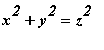 .
.
| > |
implicitplot3d(x^2+y^2=z^2, x=-3..3, y=-3..3, z=-3..3, orientation=[46, 77], axes=boxed);
|
![[Maple Plot]](images/Lesson_062.gif)
Observe that the routine has difficulties about the origin. Theoretically this can be improved by adding more points using the numpoints option. In the next section we will learn how to circumvent the problem by using a parametric representation for this surface.
Example 6.1.2
Sketch
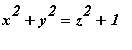 . This surface is known as a hyperboloid of one sheet and is used to design cooling towers for power plants.
| > |
implicitplot3d(x^2+y^2=z^2+1, x=-3..3, y=-3..3, z=-3..3, style=patch, orientation=[47, 79], axes=boxed);
|
![[Maple Plot]](images/Lesson_064.gif)
Example 6.1.2
Sketch the surface
 . This is known as a hyperboloid of two sheets.
| > |
implicitplot3d(x^2+y^2=z^2-2, x=-3..3, y=-3..3, z=-3..3, style=patch, orientation=[47, 79], axes=boxed);
|
![[Maple Plot]](images/Lesson_066.gif)
6.2 Parametric Representation of Quadric Surfaces
A much higher quality graphics can be obtained if we use parametric representation of the surfaces to be plotted.
Examples
Example 6.2.1
Use elliptic coordinates to plot the hyperboloid of one sheet given by:
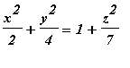 .
.
We use elliptic coordinates that transform the left hand side of this cartesian equation, into a perfect square.
| > |
elliptic_coordinates:={x=sqrt(2)*r*cos(theta), y=2*r*sin(theta)};
|

| > |
hyp_cartesian:=x^2/2+y^2/4=1+z^2/7;
|
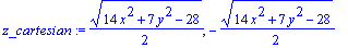
| > |
z_cartesian:=solve(hyp_cartesian, z);
|
| > |
top:=simplify(subs(elliptic_coordinates, [x, y, z_cartesian[1]]));
|
![top := [2^(1/2)*r*cos(theta), 2*r*sin(theta), (7*r^2-7)^(1/2)]](images/Lesson_0611.gif)
| > |
bottom:=simplify(subs(elliptic_coordinates, [x, y, z_cartesian[2]]));
|
![bottom := [2^(1/2)*r*cos(theta), 2*r*sin(theta), -(7*r^2-7)^(1/2)]](images/Lesson_0612.gif)
| > |
plot3d({top, bottom}, r=1..3, theta=0..2*Pi, style=patch, orientation=[37, 68], axes=boxed, labels=[x, y, z], scaling=constrained, shading=ZHUE);
|
![[Maple Plot]](images/Lesson_0613.gif)