Example 8.3.2
Find the equation of the osculating circle at the point
![P = [1, 1/2]](images/Lesson_0853.gif) to the parabola
to the parabola
 . Graph the osculating circle and the parabola in one picture.
First code the parabola as a space curve, then compute T, N and
 .
.
| > |
r:=[x, x^2/2,0];
rp:=diff(r, x);
rpp:=diff(r, x$2);
|
![r := [x, 1/2*x^2, 0]](images/Lesson_0856.gif)
![rp := [1, x, 0]](images/Lesson_0857.gif)
![rpp := [0, 1, 0]](images/Lesson_0858.gif)
| > |
T:=evalm(rp/realnorm(rp));
|
![T := vector([1/((1+x^2)^(1/2)), 1/(1+x^2)^(1/2)*x, 0])](images/Lesson_0859.gif)
| > |
Tp:=map(diff, T, x);
N:=map(simplify, evalm(Tp/realnorm(Tp)), symbolic);
|
![Tp := vector([-1/(1+x^2)^(3/2)*x, -1/(1+x^2)^(3/2)*x^2+1/((1+x^2)^(1/2)), 0])](images/Lesson_0860.gif)
![N := vector([-1/(1+x^2)^(1/2)*x, 1/((1+x^2)^(1/2)), 0])](images/Lesson_0861.gif)
| > |
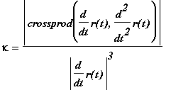
kappa:=simplify(realnorm(crossprod(rp, rpp))/realnorm(rp)^3);
|
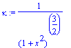
Compute
 and N at the point P.
| > |
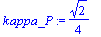
kappa_P:=subs(x=1, kappa);
|
| > |
N_P:=subs(x=1, evalm(N));
|
![N_P := vector([-1/2*2^(1/2), 1/2*2^(1/2), 0])](images/Lesson_0865.gif)
Compute the radius
 of the osculating circle.

Compute the center C of the osculating circle.
| > |
C:=evalm(subs(x=1, r)+a*N_P);
|
![C := vector([-1, 5/2, 0])](images/Lesson_0868.gif)
Compute the equation of the osculating circle.
| > |
eq:=(x-C[1])^2+(y-C[2])^2=a^2;
|
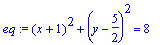
Plot the osculating circle and the parabola in one picture using the implicit plot routine.
| > |
p1:=implicitplot(y=r[2], x=-10..10, y=-10..10, color=red, numpoints=4900):
p2:=implicitplot(eq, x=-10..10, y=-10..10, color=blue, numpoints=4900):
display([p1, p2], thickness=4, scaling=constrained);
|
![[Maple Plot]](images/Lesson_0870.gif)
A higher quality picture can be obtained by parametrizing the osculating circle and using parametric plots instead.
| > |
c:=[-1+a*cos(t), 5/2+a*sin(t), 0];
|
![c := [-1+2*2^(1/2)*cos(t), 5/2+2*2^(1/2)*sin(t), 0]](images/Lesson_0871.gif)
| > |
p1:=plot([c[1], c[2], t=0..2*Pi], color=blue):
p2:=plot(x^2/2, x=-4..4):
display([p1,p2], scaling=constrained);
|
![[Maple Plot]](images/Lesson_0872.gif)
Observe that the osculating circle actually crosses the parabola at the point of tangency. This occurs because, for


 , the curvature of the parabola is larger than the curvature of the osculating circle and for
 , the curvature of the parabola is less than the curvature of the osculating circle.
It may be illustrative to show the ray from the center of the osculating circle to the point of tangency. See the picture below.
| > |
P:=subs(x=1, r);
rr:=evalm(P+t*N_P);
|
![P := [1, 1/2, 0]](images/Lesson_0877.gif)
![rr := vector([1-1/2*t*2^(1/2), 1/2+1/2*t*2^(1/2), 0])](images/Lesson_0878.gif)
| > |
p3:=plot([rr[1], rr[2], t=0..a], color=magenta):
|
| > |
display([p1, p2, p3], scaling=constrained);
|
![[Maple Plot]](images/Lesson_0879.gif)
 .
.
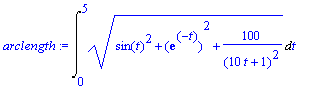
![r(t) = [cos(7*t), exp(-t), ln(10*t+1)]](images/Lesson_082.gif) , 0
, 0
 . Because T has constant length, we know that
 and therefore
 is perpendicular to T. This indicates that
 as
as
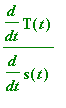 , where
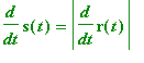 .
.
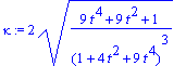
![r(t) = [t, t^2, t^3]](images/Lesson_0817.gif) .
.
![T := vector([1/((1+4*t^2+9*t^4)^(1/2)), 2/(1+4*t^2+9*t^4)^(1/2)*t, 3/(1+4*t^2+9*t^4)^(1/2)*t^2])](images/Lesson_0821.gif)
![dT_ds := vector([-2*t*(2+9*t^2)/(1+4*t^2+9*t^4)^2, -2*(9*t^4-1)/(1+4*t^2+9*t^4)^2, 6*t*(2*t^2+1)/(1+4*t^2+9*t^4)^2])](images/Lesson_0822.gif)


![[Maple Plot]](images/Lesson_0833.gif)
 .
.
 .
.
 . The Binormal vector B is defined as the crossproduct of T and N.
![T := vector([1/((1+sin(t)^2/cos(t)^2)^(1/2)), -1/(1+sin(t)^2/cos(t)^2)^(1/2)*sin(t)/cos(t)])](images/Lesson_0847.gif)