Math 173
Calculus I
Spring 2005
Dr. Constant J. Goutziers
Department of Mathematics, Computer Science and Statistics
goutzicj@oneonta.edu
Lesson 1
Maple Basics
Maple is an interactive mathematical software package which combines, Numerical Computation, Symbolic Computation and Graphics.
Initializations
Warning, the name changecoords has been redefined
1.1 Numerical Computation
All arithmetic is exact, unless we explicitly ask for a decimal approximation using the
evalf
command.
Examples
Example 1.1.1
Rational numbers, large integers, trigonometric values and decimal approximations.


Example 1.1.2
Decimal approximations of arbitrary length.
Decimal approximations of arbitrary length can be obtained by specifying the desired number of significant digits as an option in the
evalf
command. The default is ten significant digits.

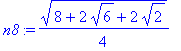
Example 1.1.3
Non-trivial trigonometric values
Some non-trivial trigonometric values can be found by using the convert to radical routine.
| > |
n8:=convert(n7, radical);
|
Exercises
Exercise 1.1.1
Compute the exact value as well as a decimal approximation of
 .
.
1.2 Graphics
Maple contains an extensive array of plotting routines, most of which can be found in the
plots
package which is loaded using the
with(plots)
command which is conveniently placed in the Initializations group at the top of this worksheet.
Examples
Example 1.2.1
The
plot
command.
| > |
plot(sin(x)/x, x=-10..10);
|
![[Maple Plot]](images/Lesson_0110.gif)
Example 1.2.2
The
color
option with the
plot
command.
We visualize the curve
 and color it blue.
| > |
plot(x^3-2*x^2, x=-2..3, color=blue);
|
![[Maple Plot]](images/Lesson_0112.gif)
Example 1.2.3
Limiting the Range of a plot.
The rational expression
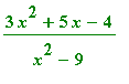 is not defined at
 and
and
 . Moreover when
 is close to either one of these values the absolute value of the expression becomes extremely large. In order to circumvent this complication, we limit the range of the plot with the option
y = -10 .. 10
.
is close to either one of these values the absolute value of the expression becomes extremely large. In order to circumvent this complication, we limit the range of the plot with the option
y = -10 .. 10
.
| > |
plot((3*x^2+5*x-4)/(x^2-9), x=-7..7, y=-10..10);
|
![[Maple Plot]](images/Lesson_0117.gif)
Example 1.2.4
Multiple plots in one picture.
We can create multiple plots within one frame by using Maple set notation
{ ... }
or list notation
[ ... ]
.
| > |
plot({x^2, 3-2*x}, x=-4..3);
|
![[Maple Plot]](images/Lesson_0118.gif)
Set notation will work with any plot routine within Maple, list notation is only implemented for some. The advantage of list notation is that it allows for control of the color of individual curves.
| > |
plot([x^2, 3-2*x], x=-4..3, color=[blue, red]);
|
![[Maple Plot]](images/Lesson_0119.gif)
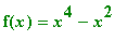
Example 1.2.5
Code and display the function
![[Maple OLE 2.0 Object]](images/Lesson_0120.gif)
Use the
piecewise
command.
| > |
f:=piecewise(x<1, 1, x>=1, 3-x);
|
![f := PIECEWISE([1, x < 1],[3-x, 1 <= x])](images/Lesson_0121.gif)
Observe that this function "jumps" at the point
 . We say that it is discontinuous at
 . Maple can be informed about this discontinuity by adding the
discont = true
option to the plot command.
. Maple can be informed about this discontinuity by adding the
discont = true
option to the plot command.
| > |
plot(f, x=-4..4, discont=true);
|
![[Maple Plot]](images/Lesson_0124.gif)
Example 1.2.6
Three dimensional images.
Maple can create three-dimensional graphs. Here is the picture of a saddlepoint surface.
| > |
plot3d(x^2-y^2, x=-5..5, y=-5..5, style=patch, axes=boxed);
|
![[Maple Plot]](images/Lesson_0125.gif)
Exercises
Exercise 1.2.1
Sketch the graph of
 and use magenta as the color of the curve.
Exercise 1.2.2
Sketch the graph of
 . Make sure that you choose the domain in such a way that the characteristics of the function around
 are clearly displayed.
1.3 Symbolics
The real power of Maple lies in its symbolic capabilities. A computer algebra system allows the user to execute mathematical computations on the computer screen much like such they used to be performed with pencil and paper. This section explores some of the capabilities of the program.
Examples
Example 1.3.1
This example illustrates the use of the
expand, factor
and
sort
commands.
| > |
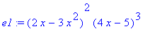
e1:=(2*x-3*x^2)^2*(4*x-5)^3;
|


Example 1.3.2
Expressions and Functions.
All computer algebra systems make a clear distinction between
expressions
and
functions
. A function has to be associated with an argument (variable).
Maple syntax for an expression g is given by: g:=expression_body; Maple syntax for a function f of variable x is: f:=x->function_body; A few examples say more than a thousand words.
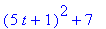
We define the expression g equal to
 as well as the function
 . Then we evaluate f` for x=a, x=2 and x=5t+1.


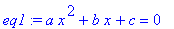
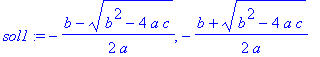
Example 1.3.3
Solve the equation
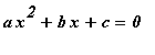 .
.
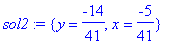
Example 1.3.4
Simultaneously solve the equations
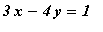 and
and
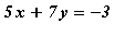 .
.
| > |
eq2:={3*x-4*y=1, 5*x+7*y=-3};
|

| > |
sol2:=solve(eq2, {x, y});
|
Exercises
Exercise 1.3.1
Compute the exact value and a decimal approximation of (1231/12)^11.
Exercise 1.3.2
Plot the graph of
 `.
`.
Exercise 1.3.3
Plot in one picture the graphs of
 and
and
 .
.
Exercise 1.3.4
Define the Maple function
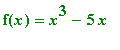 and compute
 .
.
Exercise 1.3.5
Solve the system of equations
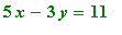 and
and
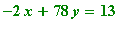 .
.