THE BIG MELT DOWN: COLUMBIA ICEFIELD, CANADA
COPYRIGHT © 2001 Paul R. Baumann
INTRODUCTION:
Approximately seventy-seven percent of the Earth’s fresh water is frozen. More than 7 million cubic miles (29 million km3) of ice covers the Earth’s surface. Most of this ice is concentrated in two places – Antarctic and Greenland. The remaining ice is spread across a few mountain ranges and alpine valleys. The fresh water ice that breaks away from Antarctica and Greenland flows directly into the oceans and mixes with salt water. This fresh water is not readily available for human use even though various plans have been proposed to move icebergs to critical areas needing fresh water. The ice located in the mountain ranges and alpine valleys feed many of the rivers that flow across the land and provide fresh water to farmlands and cities. It is these fresh water sources that society needs to monitor and protect. Most of the glaciers from these areas are melting back and many theories have been put forth as to why these glaciers are retreating. This instructional module introduces students to how satellite imagery can assist in measuring the melt back of these glaciers. The module centers on the Columbia Icefield located in the Canadian Rocky Mountains and one of the major sources of fresh water ice in North America.
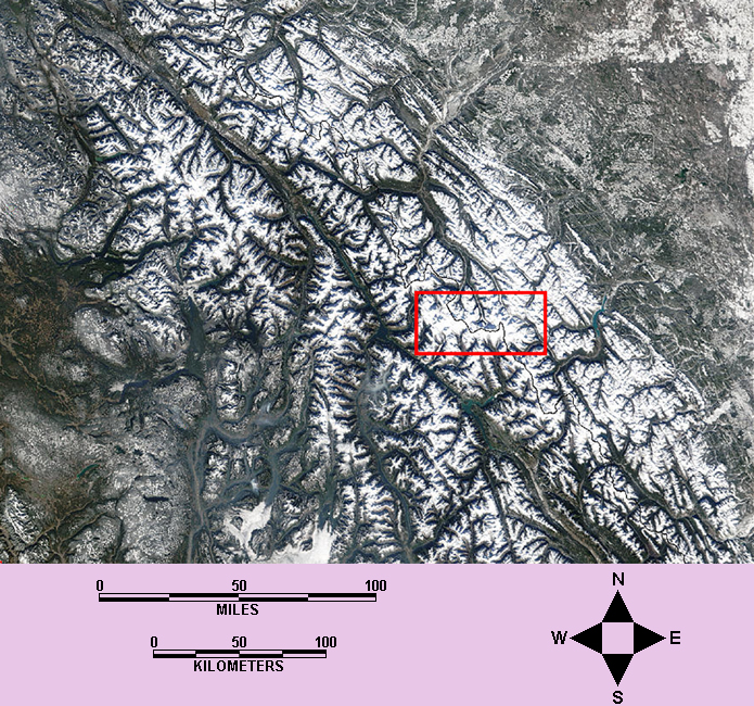
FIGURE 1: MODIS Image, taken March 4, 2002, of the Canadian Rockies with the Columbia Icefield outlined in red.
The goal of this instructional module is to measure how much certain glaciers in the Columbia Icefield have retreated over the 26 year period from 1975 to 2001. The measurements will be based on the use of four Landsat MSS, TM, and ETM+ data sets, each recorded in the late summer/early fall period. Figure 1 shows the Canadian Rockies in mid-winter with the Columbia Icefield highlighted.
BACKGROUND:
Columbia Icefield
Straddling the boundary between the Canadian provinces of Alberta and British Columbia, the Columbia Icefield is the largest ice mass in North America, south of the Arctic Circle. Situated in the Canadian Rockies, this ice field covers an area of 130 square miles (365 sq. km.) and has a maximum depth of 1,200 feet (365 m), the height of the Empire State Building in New York City. The average elevation of the ice field is about 10,000 feet (3,000 m). It occupies a high, flat-lying plateau in the form of a huge massif. Its highest points are Mount Columbia at 12,284 feet (3745 m) and Mount Athabasca at 11,452 feet (3,491 m). The average snowfall across the ice field is 23 feet (7 m) per year. Figure 2 shows the Columbia Icefield and provides the location of most of the major geographic features mentioned in this module.

FIGURE 2: General Location Map of the Columbia Icefield
Six large outlet glaciers flow from the Columbia IceField. They are the Athabasca, Castleguard, Columbia, Dome, Saskatchewan and Stutfield Glaciers. Through these glaciers fresh water flows from the Columbia Icefield into three different oceans namely the Atlantic, the Pacific and the Arctic. This situation is referred to as the "hydrographic apex of North America," basically the center of water distribution in North America. Only one other similar divide exists and it is in northern Siberia.
Meltwater from the Athabasca Glacier feeds the Athabasca River which flows into Lake Athabasca in northeastern Alberta. From this point the water enters the Slave River and Great Slave Lake to the Mackenzie River and then to the Arctic Ocean, a distance of 2,500 miles (4,000 km). Water from the Saskatchewan Glacier enters into the Saskatchewan River. From here it moves eastward crossing the provinces of Alberta, Saskatchewan, and Manitoba into Hudson Bay, and thereby, the Atlantic Ocean. These meltwaters travel a distance of 1,600 miles (2,600 km). From glaciers on the ice field’s northwestern edge, water flows into the Fraser and Columbia rivers leading to the Pacific Ocean. The Columbia River flows 1,240 miles (2,000 km) before outletting its fresh water into the ocean. If these glaciers disappear, a critical water supply, mainly for western Canada but also for other portions of North America, will be gone. To illustrate the problem, the Athabasca Glacier feeds several large prairie water systems. During the hot, dry summer of 1998, this glacier was the only thing that kept certain rivers flowing.
Glacial Landforms
Three different types of large ice masses exist, namely ice sheets, ice caps, and ice fields. Ice sheets are associated with continental glaciers and are the largest of the three types of ice masses. Today, they are found in Greenland and Antarctica. Ice caps and ice fields relate more to mountain locations. Ice caps are more circular in area and form more in a dome shape. On the other hand, ice fields are elongated in pattern and wrap around mountains leaving only their peaks showing. Such peaks are called nunatak. As its name implies, the Columbia Icefield is an ice field because it has several nunataks. All three of these ice masses have outlet glaciers around their edges that drain them to provide fresh water.
From their source to their terminus, glaciers can be divided into two zones, the zone of accumulation, and the zone of ablation or melting. Where a glacier develops near the edge of an ice field, it receives great accumulations of fresh snow. At this point the glacier appears clean and a bright white in color. The elevation is high enough and cool enough to maintain the snow throughout the year. This snow compacts as ice, which becomes part of the glacier as it moves down slope. A glacier is compacted ice that is moving. If it is not moving, it is no longer a glacier. Fresh snow and ice also enter the glacier directly from the ice field.
As the glacier flows farther away from the ice field and downhill, it becomes dirty and rougher in appearance. It is entering the zone of melting. The fresh snow is melting and exposing the glacial ice, which contains various unsorted materials. Meltwater streams appear on the surface especially during the summer. When a glacier melts more snow and ice than it receives, it begins to recede. Most glaciers in the Rockies are presently receding.
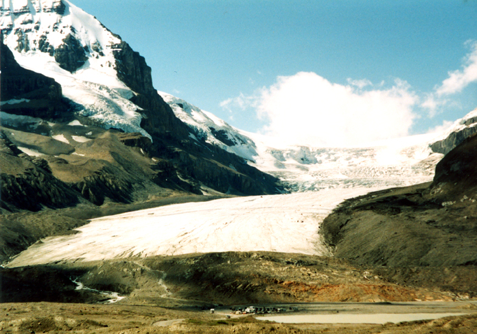
FIGURE 3: Lateral moraines from Athabasca Glacier (Photo taken August, 2001)
When a glacier recedes, large amounts of debris that has been held and carried by the ice is released and deposited on the landscape to form new landforms. This debris is referred to as till. Till is unsorted material. In other words, materials of varying sizes and shapes are mixed together when deposited. In contrast, sediment carried by running water is generally sorted with the larger materials being deposited first followed by smaller materials. Till deposited as linear ridges forms landforms called moraines. A glacier carries a tremendous amount of till near its terminus or front edge. When the glacier stops, some of this till is deposited to form an end moraine. If the glacier advances over the end moraine, the moraine might be destroyed. The end moraine that represents the farthest extension of the glacier is the terminal moraine. In the retreating process, a glacier also might temporarily stop and form a recessional moraine. As a glacier moves down a valley, the friction created by the valley sides forces deposition along the edge of the glacier. These depositions are referred to as lateral moraines. If a glacier is receding, lateral moraines provide evidence of how far the glacier has retreated. Figures 3 and 4 show Athabasca and Dome glaciers, respectively. A large lateral moraine can be observed on the right side of Figure 3. Also, a large lateral moraine can be seen cutting diagonally across the lower half of Figure 4. These lateral moraines clearly illustrate where these glaciers were previously located.
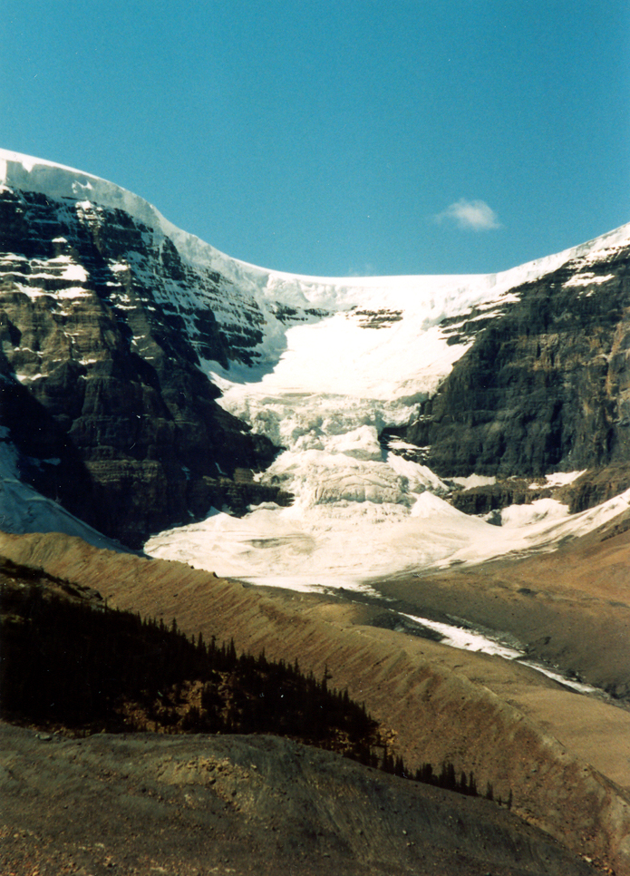
FIGURE 4: Lateral moraines from Dome Glacier (Photo taken August, 2001)
When two glaciers flow together a moraine might develop between them. This type of moraine is known as a medial moraine. The Saskatchewan glacier has a tributary glacier feeding into it with a medial moraine separating them. The brown dot pattern cutting the length of the Saskatchewan glacier in Figure 5 (Bottom) illustrates the medial moraine. This topographic map was made in 1960 and the tributary and Saskatchewan glaciers are the same length. Figure 5 (Top) shows the Saskatchewan glacier in 2001 and the tributary glacier has retreated substantially more than the main glacier. The medial moraine can be seen between the two glaciers.
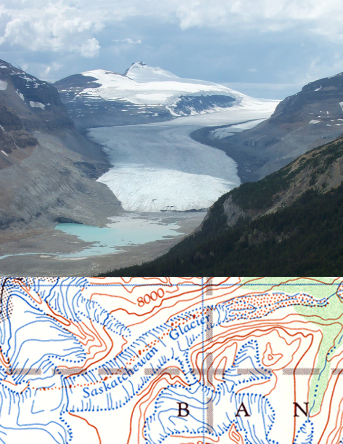
FIGURE 5: Medial moraine with the Saskatchewan Glacier
Climatic Change
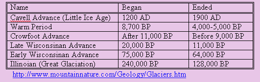
Over time the Earth’s climate has varied between cold and warm periods. Obviously, ice masses and their respective outlet glaciers expanded during cold periods and melted back during warm periods. The expansion/contraction of ice masses and the movement of glaciers have marched over the Canadian Rockies for at least a quarter of a million years. In fact, the first major ice advancement in this region may have occurred as long as 1.9 million years ago. The Great Glaciation period started 240,000 years ago and lasted until about 128,000 years ago. This period is also called the Illinoian Glaciation. Huge outlet glaciers flowed from the Canadian Rockies eastward into the central plains of present day Canada and northern United States. Their flow eastward continued until they merged with the large outlet glaciers that were rapidly expanding westward from the continental ice sheet centered over Hudson Bay. Table 1 outlines some of the major advancement and retreats of glaciers within the Canadian Rockies. Various theories as to why these glaciers started and ended have been put forth but no absolute cause has been identified. At present the Earth appears to be in a warming period as evidenced by ice masses, such as the Columbia Icefield, and their outlet glaciers melting back. Much has been written about this melt back being caused or exacerbated by various human activities, which may or may not be the case. What is known is that the Canadian Rockies have experienced several ice advancements and retreats and the present period of melt back covers a relatively short time span when compared to the last quarter of a million years.
TABLE 1: Timetable of Canadian Rockies Glacial Periods
Athabasca, Columbia and Saskatchewan Glaciers
As previously stated the Columbia Icefield has six major glaciers but this instructional module deals with only the Athabasca, Columbia and Saskatchewan glaciers. These three glaciers have been researched extensively since the early 1950s. The Athabasca Glacier presently covers an area of about 11.5 square miles (30 sq. km). The 4 mile (6.5 km) long glacier leaves the ice field at the elevation of 9,186 ft. (2,800 m), descends in a series of three ice falls as it passes over successive rock thresholds and continues as a gentile, .62-mile (1-km) wide tongue with a slope of 3-7 degrees to its terminus at 6,315 ft (1,925 m).
This glacier can be easily observed from Canadian Highway 93 and specialized buses take tourists out onto the glacier from the Icefield Centre. Investigations of its terminal, recessional and lateral moraines have recorded the movement of the glacier over the past few centuries. The glacier has advanced and retreated several times during this period. Historical records, maps, and photographs dating back to 1897 show that over the last 125 years the glacier has retreated about .93 miles (1.5 km). In 1870, the glacier was about 1.5 times its present total volume and 2.5 times its area. Tree-ring studies indicate that around 1715 the glacier had advanced more than any time in at least the preceding 350 years. The 1715 advancement would have the glacier’s terminus spreading across Highway 93 and reaching the Icefield Centre. Figure 6 shows the relative location of the glacier in 1960 to Highway 93. The Centre is located on the other side of the highway.
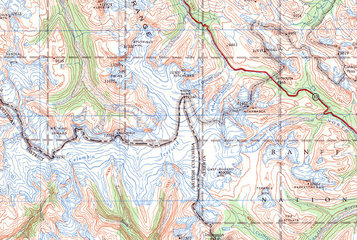
FIGURE 6: Topographic Map of Columbia Icefield (Prepared in 1960).
Figure 7 is a high-angle oblique aerial photograph of the glacier taken on August 21, 1964. The photograph shows the three ice falls coming down from the ice field. On the left side of the photograph is a long lateral moraine that provides some indication of the length and width of the glacier in the past. Next to the moraine is the road used by the specialized tourist buses and one can see where the road cut across the moraine and the buses move onto the glacier. At the bottom of the photograph are Canadian Highway 93 and the Icefield Centre. As previously stated, in 1715 the glacier had crossed over the highway and its forward edge would have occupied the present location of the Centre.
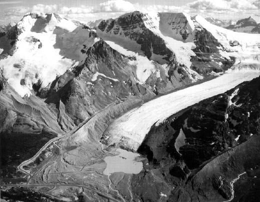
FIGURE 7: High-angle oblique aerial photograph of Athabasca Glacier taken Aug. 21, 1964 (U.S. Geological Survey)
According to research conducted by glacial scientists, the Athabasca Glacier is receding in length and shrinking in volume at an alarming rate. The melting rate is faster now than it has been in the last 40 years. Basically, the glacier is losing more moisture than the snowfall from the ice field can replace. It appears that a combination of warmer weather and a dirtier surface that absorbs the summer heat are the sources of the problem. The glacier is shrinking by 30 percent every 100 years. At this rate it will be gone in 300 years.
The Columbia Glacier, 5.28 miles (8.5 km) in length and about 6.17 square miles (16 sq. km) in area, is the major outlet glacier flowing from the northwest section of the ice field. The glacier drops rapidly from the plateau area over a major ice fall, which creates a series of very well-defined ogives (a series of ice waves formed below some ice falls). A chronological series of recessional moraines created by the glacier as it retreated has been identified, with the earliest being for 1724. The dates for the other recessional moraines are: 1842, 1854, 1864, 1871, 1907, 1909, and 1919. Between 1724 and 1924 the glacier retreated 1,292 ft (394 m), nearly one-fourth of a mile. However, from 1966 to 1977 the glacier had advanced as much as .62 mile (1 km). During this period the glacier moved forward enough to completely fill the large proglacial lake, a distance of some 2,625 ft. (800 m). The imagery associated with this instructional module shows that the glacier has been retreating again. Columbia Glacier is the least accessible of the three glaciers, resulting in less research being conducted on it.
Figure 8 is a high-angle oblique aerial photograph of Columbia Glacier. It was taken on August 21, 1964. The photograph shows a large ice fall below which is a field of waves or ogives. On both sides of the glacier wide sections of recent till deposits can be seen. Next to these deposits, steep, non-vegetation covered slopes exist. These slopes were cut by the glacier in the past and provide some idea how wide the glacier used to be. Above these slopes one can see heavy forest vegetation coverage. Small side glaciers that no longer connect with the main glacier can be observed.
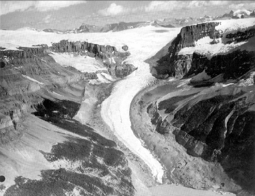
FIGURE 8: High-angle oblique aerial photograph of Columbia Glacier taken Aug. 21, 1964 (U.S. Geological Survey)
The final glacier to be studied, the Saskatchewan Glacier, is about 8 miles (13 km) long and some 23 square miles (30 sq. km) in area, making it the largest of the three glaciers. It declines gradually from east to northeast, without ice falls, to its terminus at 5,900 ft. (1,800 m). Several tributary glaciers were formerly active in providing nourishment, although by the late 1980's only one of these supplied the Saskatchewan Glacier. A small glacier runs parallel to the main glacier, separated by a medial moraine. This glacier has a different origin point. It starts from an adjacent mountain rather than directly from the ice field.
In 1953, an expedition from the American Geographical Society used photographic and botanical techniques to determine the history of the Saskatchewan Glacier. The glacier started withdrawing from its terminal moraine in 1893 and by the time of the expedition’s visit had retreated 4,475 ft. (1,364 m), an average annual rate of 75.6 ft (19.6 m). The rate of recession from 1948 to 1953 was quite fast at 180 ft. (55 m) per year.
Figure 9 is a high-angle oblique aerial photograph of the Saskatchewan Glacier. Like the photographs for the Athabasca and Columbia glaciers, it also was taken on August 21, 1964. Based on this photograph and the ground level picture (Figure 5), this glacier is massive in size. Except for in front of the tributary glacier, no great amount of till deposits exists. No lateral moraines have been developed as the glacier retreats. A vegetation line occurs along the slopes above the glacier, indicating the height of the glacier in the past. From the elevation of the vegetation line and the width of the valley, this glacier had been much larger at one time in the past. It would have been the height of the present ice field.
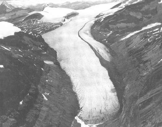
FIGURE 9: High-angle oblique aerial photograph of Saskatchewan Glacier taken Aug. 21, 1964 (U.S. Geological Survey)
ANALYSIS:
Data Sets
As stated previously four Landsat data sets are used in this exercise. Table 2 identifies the Landsat satellite, the sensor, and date for each data set. A subset for each data set was prepared. Each of the subsets has the same number of elements and lines, which makes it possible to load all of the band files into the software’s image file. Although the subsets cover basically the same geographic area, they are not geometrically rectified to each other. The spatial pixel resolution for all of the data sets is the same. The MSS subset’s spatial resolution was originally 57 x 57 m. It was changed to 28.5 x 28.5 m to make it correspond to the other data sets. Due to this change the bands are not as sharp as on the bands for the other subsets. The MSS subset also has line striping that can create some problems. It should be noted that due to seasonal weather conditions, glaciers generally move faster in summer than in winter and that the four data sets correspond in time, the late summer/early fall season. With the data sets being from the same season it makes comparisons between them easier. Also, by late summer/early fall, most of the annual snowfall has melted, which reduces the problem of separating glacial ice from annual snowfall. The software package, EarthScenes, is used throughout this instructional module and all the functions required to complete the tasks associated with this exercise are available with this package.
Table 2: Basic Comparison of the Four Data Sets
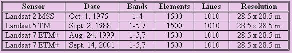
A Multiple Spectral Sensor (MSS) was available on Landsat 1, which was placed in orbit in 1972. This sensor continued to be used on the next four Landsats and recorded reflective energy in four bands of the spectrum, two visible bands and two near infrared bands. Landsats 4 and 5 launched in 1982 and 1984 had Thematic Mapper (TM) sensors that collected data in six spectral bands and one thermal band. The spectral bands covered the blue, green, and red visible and the near and mid infrared portions of the spectrum. Landsat 7 launched in 1999 had an Enhanced Thematic Mapper Plus (ETM+) sensor. This sensor had one high resolution panchromatic band that covered a wide spectral range, the same six spectral bands as the TM sensor, and two thermal bands. The TM and ETM+ spectral bands are identified as Bands 1-5 and 7. The data sets prepared for this exercise contain only the spectral bands from each sensor.
EarthScenes provides space for twenty-five input layers in its master file. If all of the bands provided for the four data sets were loaded into this file, they would occupy twenty-two of the layers and allow only three layers for various image enhancement techniques. It is recommended that only MSS bands 1-3, TM bands 2-4, and ETM+ bands 2-4 be used. This would reduce the number of band layers to twelve and provide more layers for enhancing images. However, if one has access to two computers, one can have two versions of EarthScenes operating at the same time. Two of the data sets can be loaded into EarthScenes on one of the machines and the other two data sets on the other machine. This arrangement would allow all of the bands from the four data sets to be available for use. Also, this arrangement might make it easier to compare one data set to another data set.
Procedures
The objective of this exercise is to measure how much the glaciers have retreated between 1975 and 2001. More specifically, with the use of remotely sensed imagery the objective is to measure the distance that a glacier has melted back. This can be accomplished by comparing the 1975 imagery to the 2001 imagery or by doing several shorter time interval comparisons using all four data sets. The latter approach permits one to determine if the rate of change has varied over the twenty-six year period. For illustration purposes a comparison between the 1999 and 2001 data sets of the Saskatchewan Glacier will be conducted. Using the same techniques employed in this comparison one can measure the distances between the other dates for each of the three glaciers.
First, load Bands 2, 3, and 4 for the 1999 and 2001 data sets. Since the ice and snow conditions created such a high reflectance and the mountain shadows a low reflectance, using any data stretching enhancement technique for these two data sets would not significantly improve the quality of the bands. Thus, this step can be disregarded. Next, create a false color composite image for each data set. Use band 4 for the red layer, band 3 for the green layer, and band 2 for the blue layer. Repeat this process for both data sets. Figure 10 is the false color composite image for the 1999 data set. The red color on this image represents green vegetation, predominately evergreen forest; the light brown color is mainly bare surface; medium to dark blue areas are lakes; white is the icefield; and the light blue features are glaciers. One can create different false color composite images for a data set by using different band combinations. A true color composite would be the combination of bands 3, 2, and 1 in the red, green, and blue layers, respectively. Since, as previously indicated, the data sets are not geometrically rectified to each other, one cannot use bands from different data sets to create a color composite image. Such an image would be fuzzy in appearance.
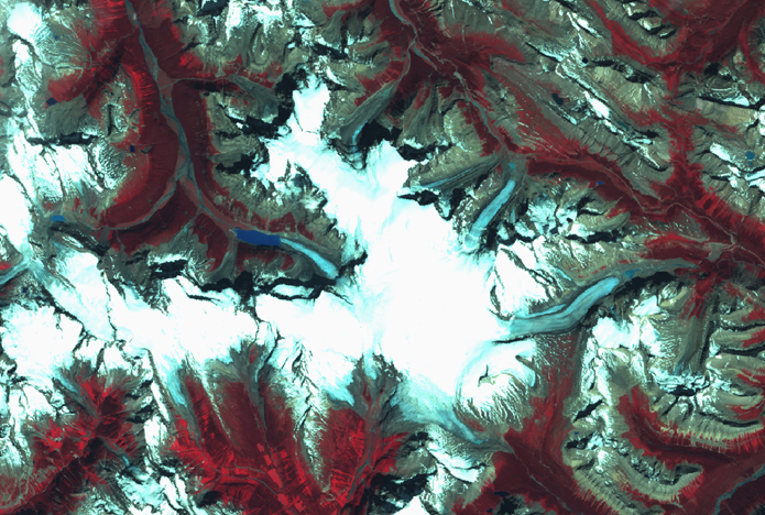
FIGURE 10: False color composite image of the study area in 1999.
Using the “Video” function on the main menu, click the “Select a window” option. The “Select an Input Layer” display will appear. Click on any band and the band image with a rectangular box will appear. Move the box on the Saskatchewan Glacier, including the area in front of the glacier and then click the mouse. This maneuver allows one to center directly on the area being examined rather than having to pan and roam every time to the desired area.
Display the false color composite for the 2001 data set. Note the various land cover and landform features along the edge of the valley. These features can be used as reference points to measure the location of the front of the glacier at different dates. It would be best to use the features on the north side of the valley since the mountains are casting shadows on the south side. Also, select features that are fixed on the landscape such as landforms; do not use features like water bodies that might vary in size. Find a feature that identifies the approximate location of the front of the glacier in 2001. For the purposes of this illustration a ravine located on the south side of the valley is used. See Figure 11 A. This feature being rather linear in nature can be continued as a line in front of the glacier. Repeat this process for the 1999 data set. In 1999 the front of the glacier is located between the ravine used with the 2001 data set and a second ravine directly to the east of the first one. See Figure 11 B.
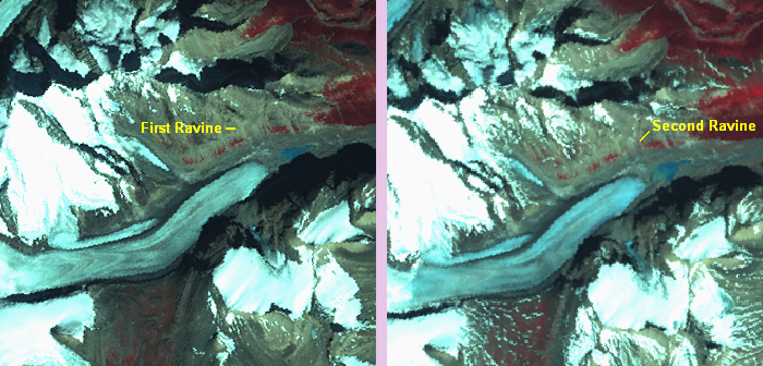
FIGURE 11 A-B: 2001 and 1999 False color composite images of the Saskatchewan Glacier.
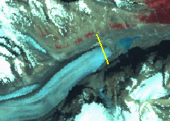
FIGURE 12: Yellow line indicates location of glacier in 2001 on the 1999 image.
Click on the “Pixel read-out and zoom” option under the “Display” menu and select the 1999 false color composite image. The portion of the image covering the Saskatchewan Glacier should appear. Using the 1999 image as a base and knowing the approximate location of the front of the glacier in 2001 (Figure 12), it is possible to measure the distance difference between the front of the glacier for the two dates. A series of numbers are displayed at the top of the “Pixel read-out and zoom” window. The first set of numbers represents the columns and rows based on the full data set and the numbers enclosed by parentheses refer to the columns and rows based on the window. As one moves the mouse across the image these numbers change. The mouse’s right and left hand buttons control the zooming of the image.
Using the 1999 image record the column and row coordinates for the front of the glacier in 1999 and 2001. The approximate coordinate location in 1999 is column 1212 and row 544 and in 2001 it is column 1204 and row 549. These coordinates can vary slightly based on where one views the front of the glacier to be for the two dates. With the coordinate values one can calculate the number of pixels between the two points by using the following formula: "C1" and "C2" represent the column coordinates for the two points and "R1" and "R2" correspond to the row coordinates.
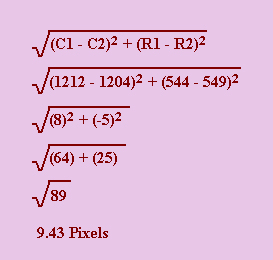
The number of pixels separating the two points is 9.43. Based on Table 2 a pixel is 28.5 meters in size; thus, the number of meters between the two points is 269.75 (28.5 x 9.43). Multiply 268.75 by 3.28 (the number of feet in one meter) to convert this distance into feet, which is 881.7 ft. Divide this number by 2 to determine the melt back rate per year (440.85 ft or 1/12 of a mile). The Saskatchewan Glacier is about 8 miles in length. At the melt back rate of 1/12 of a mile per year, the glacier should be gone in 96 years.
Notes:
In making the distance measurements one image should be established as the base image and all coordinate values should be recorded off of the base image. In the previous illustration the base image was the 1999 image. In this case if one wanted to calculate the distances between the 1999 and 1988 images, and the 1988 and 1975 images, all of the coordinate values should be taken from the 1999 image in order to avoid any geometric rectification issues that might exist between images.
The MSS 1975 image creates some challenges with respect to finding reference points. First, as previously indicated, the image is fuzzy due to its original resolution (57 m x 57 m) being adjusted to the resolution of the other images (28.5 m x 28.5 m). Second, the image contains line striping, a typical problem associated with Landsat MSS data. The striping will appear mainly over the white ice field area. Third, a diagonal line cuts across the image. It is an individual scan line problem and does not represent a problem for locating reference points. Finally, the image might appear dark. To overcome partially this problem one can enhance the bands by stretching the data. This is accomplished by using the “Contrast stretch” function. However, before using this function histograms have to be created for the appropriate bands. Use the “Create the histogram” function to complete this task.
FINAL COMMENTS:
Most people assume that clean, fresh water is readily available and all that needs to be done is to turn on the appropriate faucet allowing the water to come forth. Of course more than 70 percent of the Earth’s surface is covered by water; thus, why not take water for granted? However, only 3 percent of this water is fresh and of this 3 percent, 77 percent is frozen in icecaps and glaciers, 22 percent is groundwater; and one percent is in rivers, lakes, and wetlands. And as stated in the “Introduction” most of the fresh water from icecaps and glaciers flows directly into the salt water of the oceans. In the final analysis, very little fresh water for human use is available on the planet. As the world’s population grows, so does the demand for fresh water. Also, the water is not geographically distributed evenly throughout the world. Thus, when one of the world’s major storehouses of fresh water, the Columbia Icefield, is not providing the amount of fresh water that it used to supply it is time to determine the cause(s) of the problem and take the necessary steps to rectify the situation. Through this exercise, one can see how remote sensing can play a role in monitoring the ice field and its glaciers, a key step in analyzing the problem.
Suggested Books:
Bailey, Eric, and Kevin Van Tighem, 1987, Columbia Icefield : Ice Apex of the Canadian Rockies, Published by Minister of Supply and Services Canada Jasper, Alberta, Canada.
Freeman, Lewis R., 1925, On the Roof of the Rockies: the Great Columbia Icefield of the Canadian Rockies, New York: Dodd, Mead and Company.
Sandford, Robert W., 2003, Columbia Icefield, Altitude Publishing, Ltd.
Simmons, Lee, 1999, Jasper and the Columbia Icefield, Altitude Publishing, Ltd.
Williams, Jr., Richard S. and Jane G. Ferrigno, ed., 2002, Satellite Image Atlas of Glaciers of the World: Glaciers of North America, U.S. Geological Survey Professional Paper 1386-J, Washington D.C.: U.S. Government Printing Office.