|
|
|
|
THE ENDANGERED PENINSULAR BIGHORN SHEEP: COACHELLA VALLEY
COPYRIGHT © 2001 Paul R. Baumann
INTRODUCTION:
The Coachella Valley, which contains Palm Springs and other affluent California desert communities, is one of the best-known resort areas in the United States. Situated about 100 miles (160 km) southeast of Los Angles, its low humidity, warm winters, and abundance of sunshine attract large numbers of visitors each year. Golf courses dominate the landscape. Nearby, a tramway will take people from the warm desert environment up into the snow-covered mountains where one can ski under beautiful blue skies. See Figure 1. Tourism is the valley’s primary economic activity. It has a major convention center, numerous high quality hotels, and an airport, which is serviced by major airlines. Such a place appears to provide the ideal environment, at least for people.
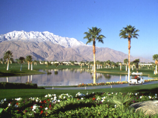
Figure 1: Palm Springs’ golf course with snow covered mountains in background.
Figure 2 provides an overview of the Coachella Valley. This Landsat 7 Enhanced Thematic Mapper (ETM+) digital image was recorded during the summer of 1999. It is a false color composite generated by combining spectral bands 4 (near-infrared), 3 (visible-red), and 2 (visible-green) as red, green, and blue, respectively. The bright red areas correspond mainly to the numerous golf courses scattered throughout the region. The mountain just east of Palm Springs is Mt. San Jacinto and the mountains in the south central portion of the image are the beginning of the Santa Rosa Mountain range. The generally dry Whitewater River cuts through Palm Springs east of the airport. The long straight line going through the center of the valley floor is Interstate 10 with a paralleling railroad line. In the northeast corner of the image is Indio Hills with the San Andres Fault line running at the base of the hills.
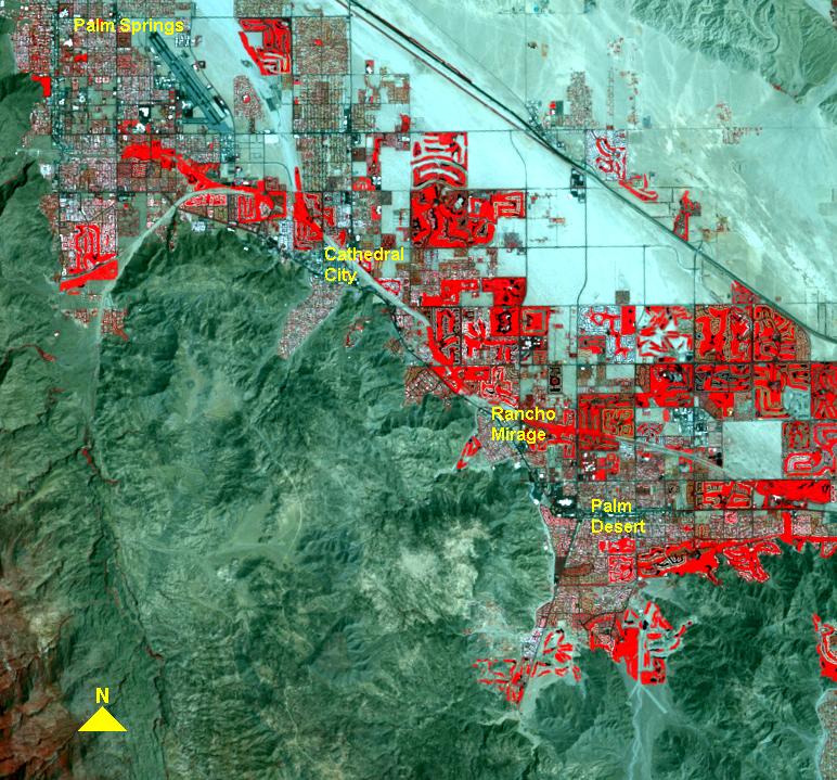
Figure 2: Landsat color composite of Palm Springs and environs.
Within this attractive environment reside the Peninsular Bighorn sheep, an animal which is on the endangered species list, and at the same time, is establishing an urban habitat. This new habitat puts it in direct conflict with the rapid urban and recreational growth in the valley. The goal of this instructional module is to develop a methodology using satellite imagery and topographic data to identify the potential sites of the Peninsular Bighorn’s new, urban habitat. This methodology employs a Landsat 7 ETM+ data set (taken July 27, 1999) and a United States Geological Survey digital elevation model (DEM) data set. These data sets encompass the area shown in Figure 2.
BACKGROUND:
This section provides relevant background information on the Coachella Valley with respect to its physical environment and population growth, the wild sheep in North America with special emphasis on the Peninsular Bighorn, the endangered species act and developers, and a small case study based on the community of Rancho Mirage. This information sets the stage for understanding the problems facing the Peninsular Bighorn and the importance for determining the potential location of their urban habitat.
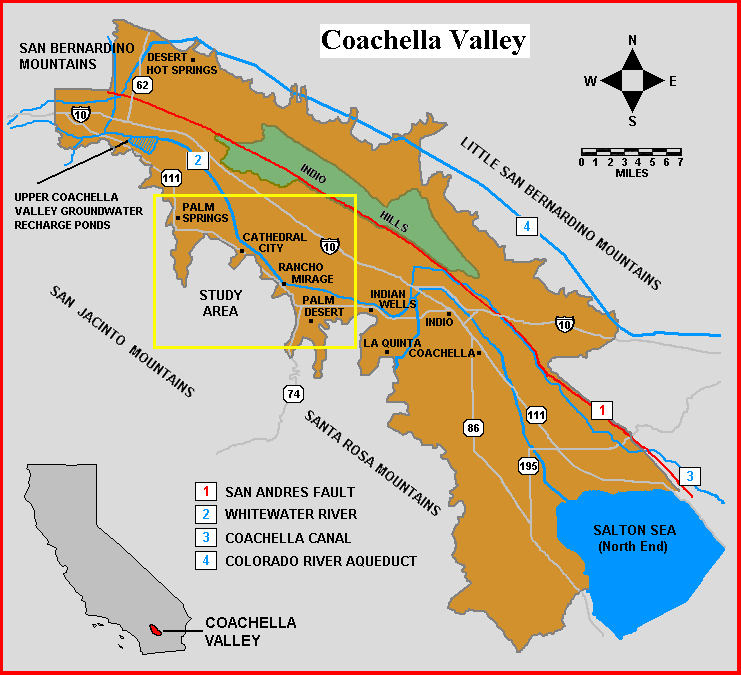
Figure 3: Coachella Valley Map.
COACHELLA VALLEY
Coachella Valley is situated northwest of the Salton Sea (Figure 3) and is an extension of the Salton Trough, a geologic depression, stretching from the valley to the Gulf of California and corresponding to the San Andres fault. A large portion of the trough is below sea level with the lowest point being -232 feet (-71m). The Salton Sea, which is in the middle of the trough, is the result of a man-made occurrence. A privately developed irrigation canal from the Colorado River into the area south of the sea, known as the Imperial Valley, could not withstand several disastrous floods on the river in 1905 and 1906 and inundated part of the region forming the sea. Since the region is below sea level, the only means for water within the sea to be removed is through evaporation. Most of Coachella Valley is slightly above sea level and is paralleled by fault-block mountains ranging in a northwest to southeast direction. The Little San Bernardino Mountains lie on the east side of the valley and the San Jacinto and Santa Rosa Mountains on the west side.
Coachella Valley is a desert with an internal drainage basin
environment. This type of environment generally consists of three major physical
realms. The first realm is the valley floor, which is relatively flat. Water, which
reaches the valley floor from the surrounding mountains, is evaporated leaving
behind alkali (salt) material. Due to this surface material and the high heat associated
with the valley bottom, the valley floor is often not a good place to live. The mountains
form the second realm. Due to their high elevation they are cooler, and thereby, have
lower evaporation rates than the valley floor. They also capture a large amount of
moisture in the form of snow. These conditions support a more lush vegetation realm
than found in the valley. Large evergreen forests cover the higher elevations. The
steep slopes of the mountains limit any high density of human occupancy. The gentle
slope areas found at the base of the mountains form the third realm. These slopes
result from sediment being carried down from the mountains by intermittent streams
and deposited at the base of the mountains. The features formed from this process
are called alluvial fans and when several fans coalesce, they create an alluvial
piedmont or apron-shaped area at the mountain base. The combination of a
gentle slope and the low level of alkali makes this realm the best for settlement in a
desert and internal drainage basin environment. Palm Springs and the other desert
communities are mainly located in this realm.
CLIMATE AND WATER
Palm Springs and the other desert communities (Cathedral City, Rancho Mirage, Palm Desert, Indian Wells, and La Qujista) of Coachella Valley are located on the leeward side of the San Jacinto and Santa Rosa Mountains. These mountains form an orographic barrier to the moist west coast winds. The valley receives an annual rainfall between 1.5 and 3.0 inches (40-75mm), and experiences extremely high temperatures and large daily temperature ranges. Table 1 shows average weather data over a sixty-five year period for Palm Springs. Annual rainfall was less than 5.5 inches during the period and several maximum monthly average temperatures reached above 100oF. The table also provides monthly potential evapotranspiration, which is the amount of moisture evaporated from the vegetation and soil. The total potential evapotranspiration is 47.77 inches, well above the total rainfall. This high evapotranspiration is due to the high temperatures and the great amount of sun. The valley never experiences a water surplus condition with respect to precipitation versus evapotranspiration. Prime evapotranspiration sites in the valley are the well-watered lawns and golf courses. Water has to be brought in from other areas via canal or obtained from groundwater.
TABLE 1: WEATHER RECORD
Palm Springs - Coachella Valley
TEMP. |
TEMP. |
TEMP. |
INCHES |
TEMP. | |
| JANUARY | |||||
| FEBRUARY | |||||
| MARCH | |||||
| APRIL | |||||
| MAY | |||||
| JUNE | |||||
| JULY | |||||
| AUGUST | |||||
| SEPTEMBER | |||||
| OCTOBER | |||||
| NOVEMBER | |||||
| DECEMBER | |||||
| PET = Potential Evapotranspiration (based on Thornthwaite) |
In 1918, the Coachella Valley Water District (CVWD) was formed to protect the valley’s limited water supply and meet future demands. In 1919, the CVWD negotiated a contract with the federal government, which provided Colorado River water for agricultural use. This arrangement conserved the valley’s groundwater supply for urban use. In 1963, the CVWD requested from the State of California its entitlements from state water projects. Rather than spending an estimated $150 million constructing an aqueduct to bring state water directly to the valley, the CVWD entered an exchange agreement with 26 other water districts along the Southern California coast. This agreement permits the CVWD to trade its state entitlement water, bucket for bucket, for Colorado River water being sent to urban areas along the coast. The Colorado River Aqueduct crosses the Whitewater River about 10 miles north of Palm Springs. The valley’s share of this water is delivered to this point. The Whitewater is just leaving the mountain area and entering the top of an alluvial piedmont where a large amount of intermittent mountain water seeps into the ground as its crosses the piedmont. In 1972 the CVWD built nine percolation ponds to increase the seepage of water from the Colorado River Aqueduct and the Whitewater. In 1984 the number of ponds was expanded to 19. Figure 4, a false-color image from the French SPOT satellite, shows the groundwater recharge ponds.
The very dark blue shown in Figure 4 is water in the recharge ponds. The Whitewater River is channeled around the north side of the recharge ponds and crosses through Palm Springs just east of the airport. One can follow the riverbed through the study area by referring back to Figure 2.
In 1936, agricultural water demand made up 87 percent of the valley’s total demand. See Figure 5. Most of this demand occurred in the southern section of the valley near the Salton Sea. This demand grew significantly until the early 1960s when it started gradually to decrease. Today agricultural demands account for about 54 percent of the water use in the valley. Municipal water use covers residential, commercial, government, and institutional demands and accounts for approximately 65 percent of the total urban demand. In 1936 these demands used 10,900 acre-ft/yr. In 1999, these demands had increased to 202,900 acre-ft/yr. Industrial use is small, less than 1 percent of the valley’s total water demand.
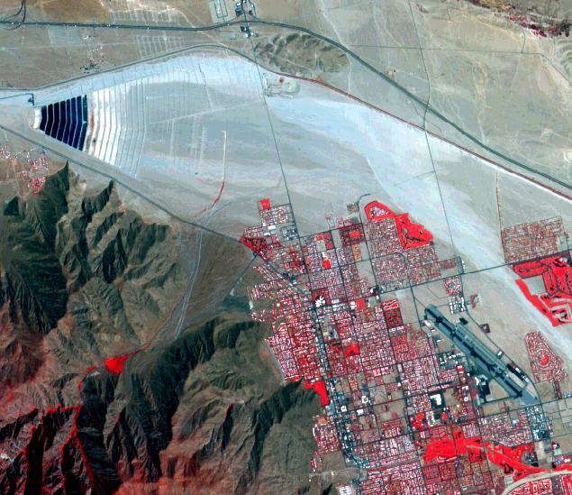
Figure 4: SPOT color composite of Whitewater ground recharge ponds.
Water use for golf courses is dramatic within the valley. Generally one does not find golf courses being compared at the same level with agriculture and urban uses. It is more of a subcategory under recreational uses within an urban landscape. The first golf course constructed in the valley was in 1925. In 1999, golf course water demand was 106,200 acre-ft/yr, one-third of the total urban demand. Most of this demand occurs between Palm Springs and Palm Desert. Golf courses and their water use play a key role in this instructional module.

Figure 5: Historical water demand by major land use
POPULATION PATTERNS
Approximately 330,000 full-time residents live in the valley. Of this number approximately 75 percent reside in nine incorporated cities with Palm Springs and Indio being the two largest cities, each with populations exceeding 48,000. Table 2, which summarizes demographic conditions in the valley is based on projections prepared by the Southern California Association of Government.
TABLE 2: POPULATION 2000
| Cathedral City | |
| Coachella | |
| Desert Hot Springs | |
| Indian Wells | |
| Indio | |
| La Quinta | |
| Palm Desert | |
| Palm Springs | |
| Rancho Mirage | |
| Unincorporated | |
| Total |
| Source: Southern California Association of Government |
Coachella Valley is projected to experience major growth over the next several decades. Between 2000 and 2035, a thirty-five year period, the valley’s population will have nearly doubled. See Table 3. The doubling rate for the entire United States is 98 years; thus, the valley is growing at a much faster rate than most of the rest of the country. This substantial population growth will result in more golf courses being created, placing pressure on water resources, and disrupting and reducing wildlife habitats. In addition to the full-time population a very large seasonal population converges on the valley. The seasonal population with second homes in 2000 was estimated to be 117,000 and this number does not include the thousands of people who come here for vacations and conferences. BBC Research and Consulting calculates that approximately 52,000 second homes exist in the valley. Many of these homes are situated in the canyons and slopes of the nearby mountains.
TABLE 3: DEMOGRAPHIC PATTERNS
| Permanent Population | |||
| Permanent Households | |||
| Seasonal Population | |||
| Seasonal Residences |
| Source: Southern California Association of Government |
WILD SHEEP IN NORTH AMERICA
In North America, wild sheep are divided into two species known as thinhorn sheep and bighorn sheep. The thinhorn sheep is further divided into two subspecies, the Dall sheep and the Stone sheep. Both subspecies are found in Alaska, British Columbia, the Yukon, and the Northwest Territories.
In comparison, the bighorn sheep have six subspecies and are found south of the thinhorn, ranging from southern Canada, through western United States into Mexico. The most abundant (31,500 - 34,500) and most widespread are the Rocky Mountain Bighorn. They are found in British Columbia, Alberta, and most western U.S. states except California. The California Bighorn, different from the Rocky Mountain Bighorn, has an estimated population of 10,500 and it ranges not only in California but British Columbia, Washington, Oregon, Nevada, Utah, and North Dakota. However, in April 1999 the U.S. Fish and Wildlife Service placed a genetically distinct population of California Bighorn in the Sierra Nevada range on the endangered list.
The most abundant desert bighorn species is the Nelson Bighorn, which number around 13,000. See Figure 6. They are located in California, Nevada, Utah, and Arizona. The next most abundant desert species is the Mexicana Bighorn with an estimated population of 6,000. They are found in the southernmost deserts of the southwestern region of the United States and the northern deserts of Mexico. The Weems Bighorn’s population is less than 1,000 and this species is only found in Baja California Sur.

Figure 6: Desert bighorn range in the United States
(Redrawn from Trefethen 1975 and Weaver 1985)
The Peninsular Bighorn, around which this instructional module is centered, are found in southern California and Baja California, Mexico. A helicopter survey taken in 1998 recorded 335 Peninsular Bighorn in the United States. Two hundred of these animals are located in Anza-Borrego Park, which is situated immediately south of the module’s study area. More recent reports indicate that the total number has dwindled to approximately 280 animals. The number of Peninsular Bighorn in Baja California ranges between 2,000 and 2,500. In the 1970s, the Peninsular Bighorn population numbered around 1,200 in the United States and between 4,500 and 7,800 in Baja California. The population in the United States has decreased by 72 percent since the 1970s. In 1971 the state of California identified these animals as being threatened, and in 1998 the U.S. Fish and Wildlife Service placed the Peninsular Bighorn on the endangered list.
PENINSULAR BIGHORN
The Peninsular Bighorn’s traditional habitat is the rocky, dry, low elevation slopes, canyons, and washes associated with the San Jacinto and Santa Rosa mountains adjacent to Palm Springs, California and extending south into Baja California, Mexico. See Figure 7. Their habitat has changed dramatically within the last thirty years due to a variety of interrelated factors. One such factor is the mountain lion. Urbanization on the West Coast from Los Angeles to San Diego has been moving eastward into the mountains putting pressure on the regular habitat of the mountain lion. More people living in the exurbia regions of these large cities are reporting having mountain lions in their backyards. What these people fail to realize is that the mountain lion is not moving into their backyards but that they have moved into the mountain lion’s front yard. This pressure has resulted in some mountain lions moving farther eastward into the mountains creating a high density of animals. In addition, the number of lions has increased since 1991 when California made it illegal to hunt them.
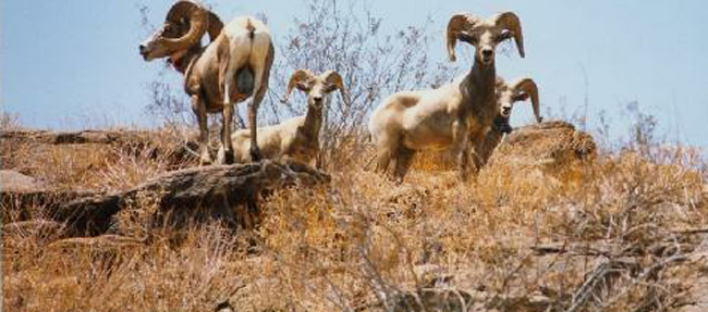
Figure 7: Peninsular Bighorn Sheep in their natural habitat.
(Photo from Bureau of Land Management)
With increased numbers and expansion of urbanization, the mountain lion has become a more active predator impacting the bighorn’s population. In a recent three-year period over 40 radio-collared sheep in the Anza-Borrego Park were killed by lions. The problem is severe enough that any lion observed killing a bighorn will be shot even though it is illegal to kill them.
The lion and urban expansion has forced the bighorn to find a new habitat in the lower elevations near Palm Springs and other communities along the eastern edge of the Santa Rosa mountains. This new habitat consists of the lush, green vegetation associated with the well-watered golf courses and residential areas, which are abundant throughout the affluent desert communities. There are many seasonal homes located near the mountains that have large lawns and swimming pools. Being seasonal, they are frequently quiet areas, which make them even more attractive habitats. Caretakers often find sheep grazing on lawns, eating plants around homes and drinking water from the swimming pools. See Figures 8 and 9.
This new habitat brings the sheep into contact with the automobile, other human settlement conditions, poisonous plants, and parasites. The Bighorn Institute reported that between 1991 and 1996 in the northern Santa Rosa Mountains, five bighorn were killed by cars, one strangled in a wire fence, and five died from eating poisonous ornamental plants. The Institute further indicated that 34 percent of the adult bighorn mortalities during the six year period associated with its report were due to urbanization, making it the leading cause for the death of bighorn in the Palm Springs area. Read the new release, “Urbanization: a leading cause of bighorn mortality,” which is attached at the end of this module.
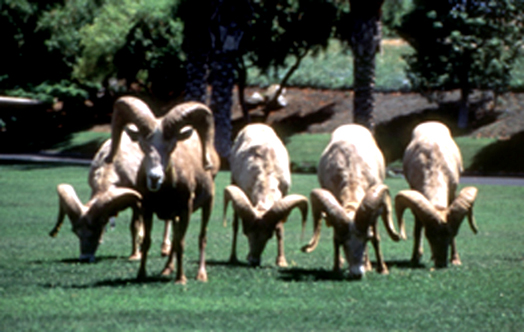
Figure 8: Do you need your lawn cut? Call Bighorn Lawn Service.
(Caption by author; photo by the Bighorn Institute)
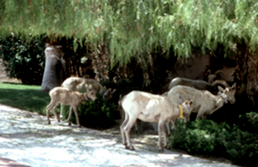
Figure 9: Is this where the party is being held?
(Caption by author; photo by the Bighorn Institute)
In 1991, the Sierra Club petitioned the federal government to place the Peninsular Bighorn on the endangered status list but developers effectively fought the petition until 1998 when the petition was finally approved. Even though Peninsular Bighorn was placed on the endangered species list, the Southwest Center and Desert Survivors had to file a suit against the U.S. Fish & Wildlife Service in order to get the agency to designate the critical habitat for the Peninsular Bighorn. The law requires the agency to identify and protect specific critical habitat for each endangered species but the agency will not act unless sued. The agency listed 179 species under the Endangered Species Act between 1996 and 1998, and in each case, did not designate critical habitat. Under the law, critical habitat designation requires protecting an ecosystem even though a species might not be currently present. Developers and some legislators find this aspect of law difficult to accept.
Finally, in response to a court order, the U.S. Fish and Wildlife Service designated 844,897 acres of land in portions of San Diego, Imperial, and Riverside counties, California as critical habitat for the endangered Peninsular Bighorn. Most of the area designated is under local, state or Federal jurisdiction, and includes portions of the Anza-Borrego Desert State Park, and lands under the Bureau of Land Management and the U.S. Forest Service. Nearly 130,000 acres of private land fall under the final critical habitat designation.
Under the Endangered Species Act, critical habitat is defined as:
“specific geographic areas that are essential for the conservation of a threatened or endangered species and may require special management considerations. These areas do not necessarily have to be occupied by the species at the time of designation. A critical habitat designation does not set up a preserve or refuge and only applies to situations where Federal funding or a Federal permit is involved. It has no regulatory impact on private landowners taking actions on their land that do not involve Federal funding or permits.”
In its final designation report, the Service removed approximately 30,700 acres of land included in the proposed critical habitat designation published earlier. Some lands originally proposed were excluded from the final designation because the Service was able to more precisely map areas that contain habitat essential for the conservation of the bighorn. The more precise mapping made it possible to eliminate many significant urban or developed areas that no longer contain the physical and biological features necessary to support the species. Some of the lands removed from the critical habitat boundaries include urban interface areas in the Coachella Valley from Palm Springs, east to La Quinta. The problem that this approach does not address is, “What happens when a species changes its habitat?” What happens when a species’ habitat becomes golf courses and people’s yards rather than the natural environment?
The battle over the Peninsular Bighorn involves big money. House lots in Palm Springs and other desert communities are selling up to $1 million per acre. New golf- resort communities are moving up into the nearby canyons since most of the prime land for golf course development is already taken. These canyons are key habitat areas for the bighorn. Jim DeForge of the Bighorn Institute likes to point out that Palm Springs and the other desert communities already have 100 golf courses, more courses than bighorn in the immediate area. Ironically, one developer, who converted several hundred acres near Palm Desert into a golf-resort community, named it Bighorn and placed statues of bighorns near the entrances. In the near future these statues might be the last place that people can see the Peninsular Bighorn.
Under the Endangered Species Act of 1973, the U.S. Fish & Wildlife Service can significantly change a development project if the project threatens the habitat of the Peninsular Bighorn. Mark Bragg, president of Shadowrock Development Corp., is fully aware of this situation. In 1998, he was informed that he had to contribute 100 acres of his project to protecting the bighorn habitat and donate $500,000 to assist in mitigating development intrusion into the habitat. Four years before the State of California required him to donate 600 acres of a 900 acre development and $500,000 for mitigation. Mr. Bragg has now organized what he calls “victims of the U.S. Endangered Species Act” as a way to stop the federal government from financially injuring people when protecting endangered species. He points out that only 280 Peninsular Bighorn exist in a 10,000 square mile area between Palm Springs and the Mexican border. How much and what type of space do they need for these few animals?
RANCHO MIRAGE
In recent years the Peninsular Bighorn Sheep have been active in the canyon behind Rancho Mirage. Rancho Mirage is a resort community of wealthy retirees. According to the 2000 U.S. Census of Population the median population age for Rancho Mirage is 61.3 years, which clearly identifies it as a retirement area. The median age for a more typical community ranges between the high twenties and low thirties. The full-time residential population for Rancho Mirage is 13,249 and the total number of houses is 11,816, almost one house per person. However, only 6,813 of these houses are occupied during the entire year. The majority of the remaining 5,003 houses are seasonal or recreational homes, basically second homes. Such a high percent of second homes indicates a certain degree of wealth. The major economic activities in the community are health care facilities and tourism with a number of nice conference hotels and golf courses. The four largest employers are the Eisenhower Medical Center, including the Barbara Sinatra Children's Center and the Betty Ford Clinic, (1800 employees), Westin Mission Hills (620), Marriott Rancho las Palmas (500), and Ritz Carlton (375).
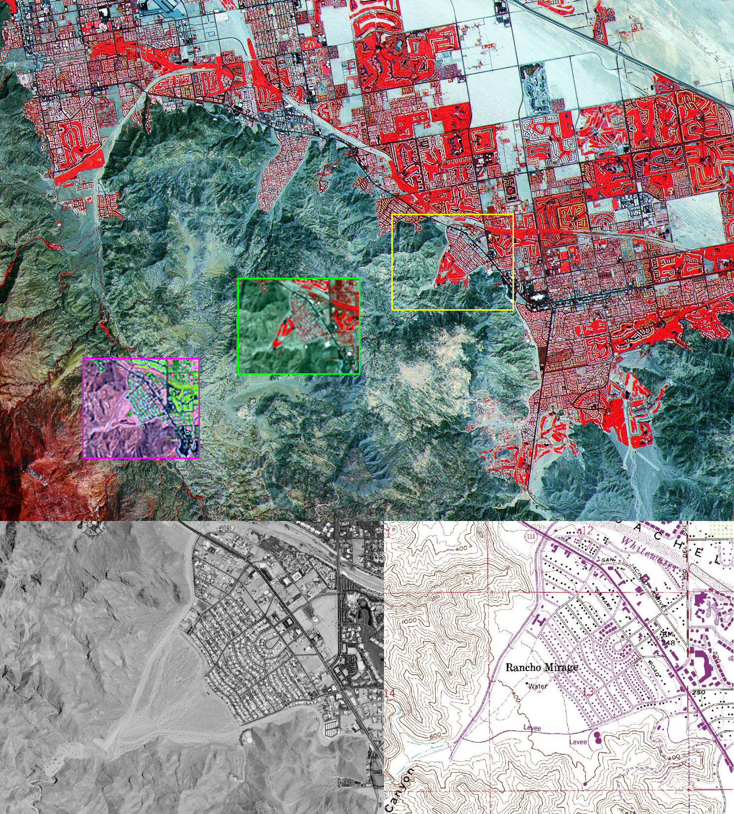
Figure 10: Rancho Mirage shown on aerial photography, topographic map, and satellite images.
Click on image to view full scale image.
This golf course with its water areas and surrounding homes, many
of which are seasonally occupied, is an attractive area for the bighorn sheep. Rancho Mirage
is now in the process of building a large retaining fence around the upper canyon in order to
keep the sheep from coming out of the mountains. Cars along Highway 111 in the Rancho
Mirage area have struck at least 10 bighorn of which 6 were killed. Rancho Mirage should be
recognized for its efforts in trying to protect the bighorn but fences require constant maintenance
and are not always successful in keeping things out. The hope is that the fence will change the
sheep’s behavioral patterns and they will stay in their traditional habitat. However, an examination
of Figure 10 clearly shows several other areas similar to Rancho Mirage where the sheep have easy
access to golf courses and water. It will not be feasible to separate the entire valley from the
mountains with a fence.
ANALYSIS:
DATA SET
On April 15, 1999, Landsat 7 was successfully placed into orbit and its Enhanced Thematic Mapper Plus (ETM+) started recording images. The main data set used in this instructional module comes from an ETM+ image recorded on July 27, 1999. It is 719 lines by 772 elements in size. The software package, EarthScenes, is used throughout this module and all the functions required to complete tasks associated with this module are available in this package.
An ETM+ data set has eight bands. Six of the bands are identical to the Landsat 4 and 5 Thematic Mapper reflective bands. They cover the same spectral range and have the same spatial resolution of 30m by 30m. These spectral bands are 1-5 and 7. The thermal infrared band, Band 6, found on the TM scanner is also available but its spatial resolution has increased from 120m by 120m to 60m by 60m. It covers the same spectral ranges; however, the data have been provided in low and high gain, making for two bands, Band 6L and Band 6H. Finally, there is a new panchromatic band, which has a wide spectral range extending from the green visible through the near infrared portion of the spectrum. This band has a spatial resolution of 15m by 15m. The panchromatic and thermal bands are not included with the data set provided for this module. Certain technical problems exist in trying to convert them to the same resolution as the six basic bands.
In addition to the Landsat data set, a topographic data set is being provided. This data set has three layers, namely elevation, slope, and aspect. These topographic layers are at the same resolution as the ETM+ bands and are geometrically rectified to them. This data set was obtained from a United States Geological Survey (USGS) digital elevation model (DEM) for the Santa Anna 1:250,000 topographic map. DEM data are arrays of regularly spaced elevation values referenced horizontally either to a Universal Transverse Mercator (UTM) projection or to a geographic coordinate system. The grid cells are spaced at regular intervals along south to north profiles that are ordered from west to east. Since a 1:250,000 USGS topographic map covers an area of two degrees longitude by one degree latitude, two DEMs are created for each map, one for the eastern half and the other for the western half of the map. Each of these DEMs is organized into a grid of 1201 rows by 1201 columns and an elevation value is determined for each grid cell. Surfer 7.0, a sophisticated terrain modeling software package developed by Golden Software, was used to interpret the DEM for the eastern half of the Santa Anna topographic map. It rescaled the elevation data to the scale of the ETM+ bands and produced slope and aspect values from the new elevation data. This data set is 719 lines by 772 elements in size.
Since EarthScenes, like most image processing software packages, is designed to handle satellite data, the data range is expected to be 0 to 255. The topographic data had to be converted to this range. Thus, one should not view the elevation data with respect to being in feet or meters but on a scale of 0 to 255. The same holds true for slope, which was originally calculated as percent of slope with the maximum possible slope being 90 percent. Aspect is also at the scale of 0 to 255 but unlike elevation and slope, aspect is an arbitrary code number representing the direction a slope is facing.
NDVI
Since the bighorn sheep are seeking habitats with good green vegetation, the first step is to locate such areas on the imagery by using a technique called the Normalized Difference Vegetation Index (NDVI). The NDVI is determined using the reflected solar radiation in the near-infrared (NIR) and red (RED) wavelength bands. NDVI values vary with absorption of red light by plant chlorophyll and the reflection of infrared radiation by water-filled leaf cells. Thus, in most cases, NDVI relates with photosynthesis. Since photosynthesis occurs in the green sections of plant material, the NDVI is generally used to identify green vegetation. The formula for creating the index is:
NDVI = (NIR - RED)/(NIR + RED)
Band 3 deals with the red visible portion of the electromagnetic spectrum and Band 4 the near infrared portion; thus, they will be used to create the NDVI for the study area. In EarthScenes, the NDVI can be produced by going to the “Arithmetic operations on layers” function under the “Enhance” menu and clicking on “Window and layer processing” and “Output 9.” The formula for “Output 9” is:
(C1*P1 + C2*P2)/ (C3*P3 + C4*P4)
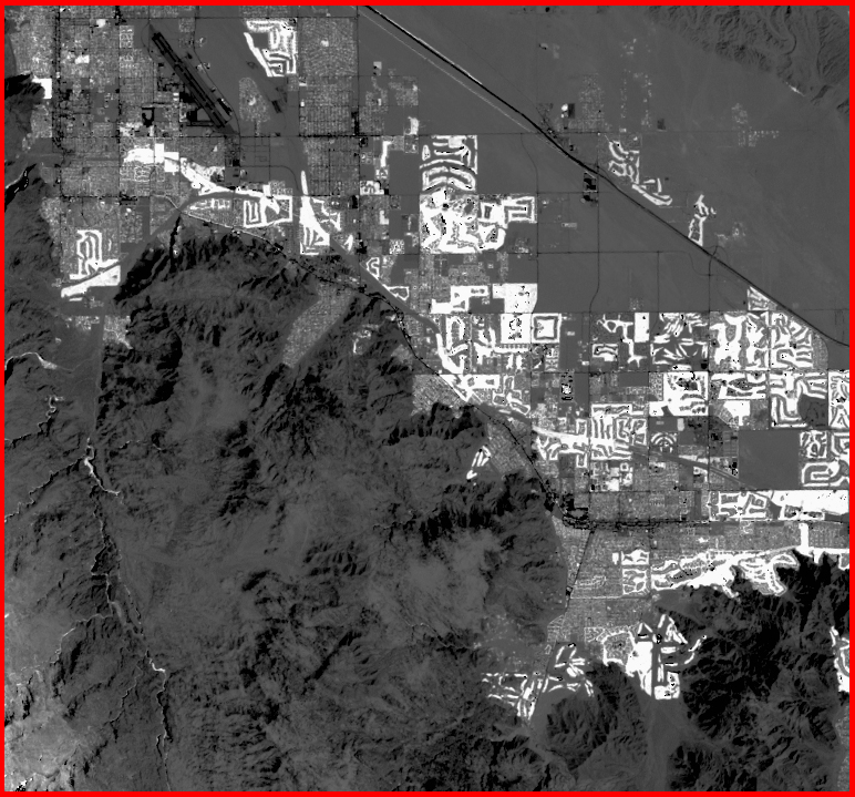
Figure 11: NDVI Image
In the formula, the letter “C” relates to a constant and the letter “P” to a pixel in a layer in the image file. The formula should be:
(1*Band 4 + (-1)*Band 3)/ (1*Band 4 + 1*Band 3)
Note that the constant is “1” in each case except one where it is “-1.” The program expects bands 4 and 3 to be entered twice. The output should be scaled into the range of 1-250. The very bright (white) areas on the new image, Figure 11, are the areas with green vegetation. Golf courses are very clearly identified.
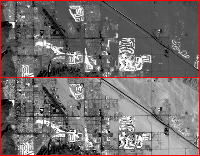
Figure 12: NDVI image (top) and Band 4, (bottom).
However, in comparing the NDVI layer (Figure 12, top) to Band 4, (Figure 12, bottom), one might conclude that Band 4 is already identifying the green vegetation area, which would raise the question as to why go through the process of creating the NDVI. A closer examination of the two pictures will show that some significant differences exist. First, some of the bright areas shown on Band 4 do not appear as bright on the NDVI layer. These areas are not covered with green vegetation. Second, on Band 4, a number of black dots appear on the golf courses. These are ponds or water traps. Near infrared is very good at separating water from land. These dots on the NDVI layer are much smaller and some have disappeared. The edges of these ponds are generally shallow and aquatic plants have taken root. One would find it difficult to identify these areas as being either water or land. Third, the NDVI process smoothes out information. The mountains and urban areas are much more defined on Band 4 than on the NDVI layer. Although this loss of detail might appear to be a problem, it will become a benefit when the NDVI layer has to be separated into different land classes. For the purposes of this project, the NDVI layer is better than Band 4.
DEM DATA
The NDVI layer shows green vegetation areas extending from the edge of the mountains out to the middle of the valley. The bighorn sheep depend upon the ruggedness of the mountains to help protect them. Although they might enjoy the green vegetation and water areas of the valley, they are reluctant to venture far into the valley away from the protection of the mountains. The next step in identifying the new habitat for the bighorn sheep is to separate those green areas near the mountains from those farther out in the valley. Here is where the topographic data can be used. Since this portion of the analysis involves separating those green areas near the mountains from those near the valley, it would appear reasonable to use the elevation layer in the data set. Areas near the mountains will have higher elevations than areas in the valley floor.
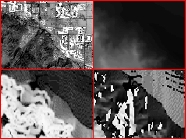
Figure 13: Band 4 (upper left), Elevation (upper right), Slope (lower left), and
Aspect (lower right).
However, the entire valley is sloping gradually down from the northwest to the southeast. A given elevation in the higher northwest portion of the valley will be farther away from the mountains than the same elevation in the lower southeast section of the valley. In order to maintain the same distance away from the mountains, the desired elevation level would have to change as it moves through the data set, something hard to accomplish and not within the capabilities of the software.
Based on the problem just outlined with respect to elevation, slope might appear to be a better choice since it plays an important role in urban growth and development. However, humans are noted for reshaping the land. For example, it is desirable for golf courses to be relatively flat. To accomplish this condition for courses located near the mountains, slope conditions have to be changed. Thus, these courses with their nice green grasses that attract bighorn sheep have slopes similar to those in the valley floor. Separating relatively flat slopes at different elevations would be very difficult. Also, natural terraces exist on mountainsides resulting in small flat areas. Aspect, the direction in which the slope is facing, introduces another set of problems mainly related to the fact that the numerical values in this data layer are artificially assigned code numbers.
Thus, the basic question is, “Which one of the three topographic attributes should be used in this project.” At this point, it might be desirable, spatially, to compare elevation, slope and aspect to one of the spectral bands. In Figure 13, Band 4 (upper left) shows Cathedral City and a number of golf courses in the valley. With white representing high elevations and black low elevations, one can observe a correlation between elevation (upper right) and the features displayed on Band 4. On the other hand, slope (lower left) appears to be a variety of texture patterns, and may be initially, difficult to perceive. White indicates steep slopes and black low slopes. The mountains show many different shades of white, which should be expected due to the changing slope conditions found in this type of environment. The valley floor is only displaying a few dark colors, typical in areas with little variation in slope. The alluvial piedmont or apron area at the base of the mountains is well defined by the medium gray shades. Aspect (lower right) shows in white slopes facing west and in black facing east. One can see a relationship between aspect and the mountains shown in Band 4. It is much harder to note any relationship when observing the valley. Since people, in general, are more accustomed to noting elevation differences than slope and aspect changes when observing the landscape, elevation will be used.
CLASSIFICATION
The next step in this project is to analyze and classify the NDVI and Slope layers. The NDVI classification is relatively simple since it will be a two-land cover classification - low-density vegetation and high-density vegetation. The term “low-density vegetation” refers to areas with sparse vegetation and the lack of greenness in the vegetation; whereas, “high-density vegetation” surfaces contain lush vegetation with high levels of greenness.
First, under the Enhance menu, one needs to create a histogram of the NDVI layer. After the histogram has been created, it might be interesting to plot it in order to obtain some idea about the distribution of the data. Second, under the Display menu, a pixel read-out of the NDVI layer must be done. Moving the cursor across the layer, the z-value for each pixel will be displayed. Determine the z-value range for the vegetated areas. The boundary between the high-density and low-density vegetation areas is generally an educated judgment determination. The z-value range selected by this analyst for the high-density vegetation areas was 216 to 250. Finally, under the Classify menu, a density slice classification of the NDVI layer is created. Following the instruction provided, one selects Window and Layer Processing and makes a two-land cover classification with the low-density vegetation class ranging from 1 to 215 and the high-density vegetation class from 216 to 250. See Figure 14. A new layer will be created, which will have values of 1s and 2s representing the two classes. See Figure 15. Also, a numerical count of the number of pixels in each class will be provided. These numbers were 528,807 and 26,261 for class 1 and 2, respectively. With this information, the amount of area in each class can be determined.
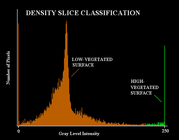
Figure 14: Density Slice of NDVI Histogram.
The area measurements in Table 4 were ascertained by first determining the number of square feet in one pixel. One meter equals 39.37 inches or 3.28 feet. The number of feet, 3.28, is multiplied by the number of meters along one side of a pixel, which is 30 for the ETM+ data. This calculation provides the number of feet along one side of a pixel, which is 98.4. This number is squared to obtain the total number of square feet in one pixel (9,682.56), which is then divided by 43,560, the number of square feet in an acre, to determine the proportion of an acre covered by one pixel. This proportion (0.222281) is finally multiplied by the number of pixels in each land cover class to obtain the number of acres in each class. For example, the number of acres in the high-density vegetation class equals: 0.222281 x 26,261 pixels, or 5,837 acres. Multiply the number of acres by .4047 to obtain the number of hectares. Divide 640 into the number of acres and 100 into the number of hectares to get square miles and square kilometers, respectively.
TABLE 4: NDVI CLASSIFICATION RESULTS
| Low-density vegetation | |||||
| High-density vegetation |

Figure 15: NDVI Classification - Low-density vegetation (Brown) and
High-density vegetation (Red).
The next step is to perform a density slice classification on elevation. The procedures involved are the same as used in classifying the NDVI. The data values for elevation range from 7 to 150, or roughly 200 to 6900 feet. The data values are in integer form, and as indicated previously, are limited to a range of 0 to 255. Each integer value represents approximately 47 feet. The full range of 0 to 255 is not used since the data set was taken from a larger data set, which had a larger elevation range.
To assist in working with elevation, the data are first stretched using 7 to 102 as the lower and upper levels. In the stretching process, the values of 7 and 102 and above are assigned to 1 to 250, respectively. Not many values exist from 102 and above; thus, compressing them will not result in much of an information loss. EarthScenes limits the data range from 1 to 250 rather than 0 to 255. Figure 16 illustrates the difference between the normal and stretched elevation data. The stretched data provides a better picture of the elevation condition.

Figure 16: Normal Elevation (left) and Stretched Elevation (right).
The piedmont is the principal area of interest for this project. This is the area where people and most of their settlement activities are occurring. Since no empirical information exits as to how far the bighorn sheep traverse from the protection of the mountains into the urban vegetated areas, the piedmont was divided into two areas: the lower slopes and the upper slopes. The upper slopes, the areas nearest the mountains and with the highest urban development, represent the best location, topographically, for the urban habitat of the bighorn sheep.
To select the boundary between the lower and upper slope areas, the pixel read-out function needs to be employed. The gray-tone picture of the stretched elevation provides few reference points from which to select a boundary. To overcome this problem, a color composite can be created by assigning the stretched elevation data to the red color and Band 4 to both the green and blue colors. Figure 17 shows this color composite. Using the pixel read-out function, one can see how the elevation values (red) change in reference to the landscape, which is provided by the information from Band 4. As one moves the cursor, not shown in Figure 17, across the screen, the elevation values will change according to the landscape. A key feature on the landscape is route 111. This road forms a barrier for the bighorn sheep to cross and some of them have been hit by vehicles in trying to reach the other side of the road. Route 111 will be used in determining the boundary between the lower and upper slopes of the piedmont. The green areas of the upper piedmont between the mountains and route 111 represent the best urban habitat for the sheep. After trying several different elevation boundaries, this analyst found the value of 20 to provide the best results. Going below this level resulted in some green areas far out in the valley floor appearing. Values above this level produced very few areas of the desired green urban habitat. The value of 20 corresponded in many sections to route 111.
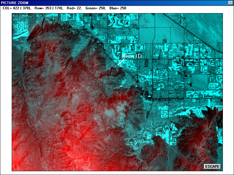
Figure 17: Pixel Read-Out Color Composite.
With the value of 20, a density slice classification can be done on the stretched elevation data. The number of pixels counted for the area of 20 and below was 238,296 and for the area above 20 the number was 316,772. These values can be converted into area measurements similar to what was done with the NDVI classification. Figure 18 shows the graphic results of this classification.
The final step in this analysis is to bring together the NDVI and stretched elevation classifications to create a new classification. Both classifications contain values of only 1s and 2s since they are each based on two classes. To merge these two classifications by adding them together would not result in four distinct classes since mathematically some of the combinations would produce the same numerical values. To overcome this problem, the NDVI classification is multiplied by 10. This mathematical step is done in EarthScenes by using option 2 under Arithmetic Operations. This modified NDVI classification and the stretched elevation classification can now be added together to produce yet another new classification. It is important to truncate the output range rather than scale it between 1 and 250 when doing this addition. This new classification will have values of 11 and 12, that relate to low-density vegetation areas, and values of 21 and 22, that cover high-density vegetation areas. The value of 21 corresponds to high-density vegetation areas at lower elevations and 22 to high-density vegetation areas at upper elevations.

Figure 18: Elevation Classification.
This new classification can now be divided into four classes by doing a density slice. However, since the low-density vegetation areas are not relevant to this analysis, they can be grouped into one class. Once the results of the classification have been generated, it might be best to display the results in a different color table than the default classification color table in order to neutralize the color assigned to the low-density vegetation areas. A new color table can be created under the Look-up-tables menu. Figure 19 shows the new classification with a different color table. The gray corresponds to the low-density vegetation areas. Red and yellow relate to high and low elevation areas, respectively, with high-density vegetation surfaces.
Figure 19: Final Classification.
Table 5 provides the area measurements for these three surfaces. As a last step this final classification is stretched with class 1 being assigned to 1 and class 3 to 250. A color composite is then created with the stretched classification being red and Band 3 being both green and blue. Figure 20 is this color composite with the bright red areas being the potential urban habitats for the Peninsular Bighorn sheep in the Coachella Valley.
TABLE 5: FINAL CLASSIFICATION RESULTS
| Low-density vegetation | |||||
| Low elevation | |||||
| High elevation |
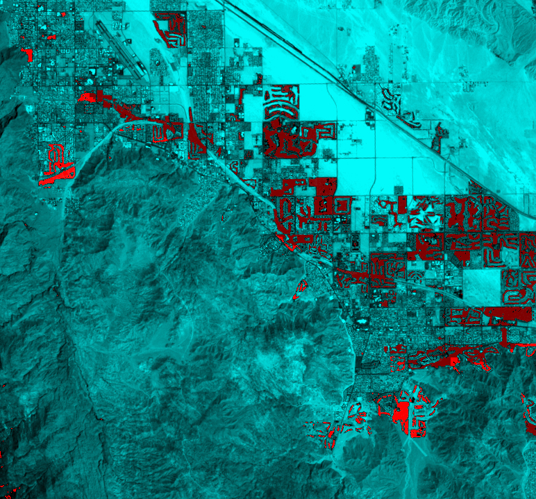
Figure 20: Color Composite with Final Classification and Band 3.
Bright red represents the potential urban habitat areas for the Peninsular Bighorn Sheep.
ATTACHMENT:
The following are exerts from
THE BIGHORN
Official Newsletter of the Bighorn Institute
Urbanization: a leading cause of bighorn mortality
The northern Santa Rosa Mountains (NSRM) border the cities of Cathedral City, Rancho Mirage, and Palm Desert in Southern California. Since 1981, Bighorn Institute (BI) has closely monitored radio-collared bighorn in this area to determine causes of adult bighorn mortality. Bighorn in this study wear radio-collars containing mortality sensors which are triggered when the animal does not move for four hours. Whenever BI biologists detect an animal on mortality mode, they locate the bighorn as soon as possible to investigate the cause of death. If the animal is located within 36 hours of its death, and biologists are unable to determine the cause of death, the carcass is transported to the California Veterinary Diagnostic Laboratory in San Bernardino, California for a necropsy (autopsy).
Between 1991 and 1996, we recorded 32 adult bighorn mortalities in the NSRM. Of these, 11 (34%) were directly caused by urbanization, 9 (28%) were caused by mountain lion predation, 1 (3%) by disease, and 11 (34%) were caused by unknown factors or old age.
Our data shows that bighorn sheep in the NSRM often find themselves in peril at the urban-mountain interface. During the six year study period, we documented 9 bighorn hit by automobiles, 5 of which were fatally injured; 5 bighorn deaths from ingestion of exotic poisonous plants such as oleander; and 1 bighorn strangled in a wire fence. In addition to these direct effects, urbanization may affect bighorn sheep indirectly by altering their habitat use, diet, and behavior, making them more prone to parasite infestation and potentially more susceptible to predation. The NSRM bighorn herd is notorious for low lamb recruitment, and factors associated with urban areas may be contributing to this serious dilemma. High levels of internal parasites have been detected in desert bighorn that graze in unnaturally moist environments, such as residential areas within bighorn habitat.
Problems found in both the NSRM and the San Jacinto Mountains (bordering Palm Springs, California) are analogous to those in the Pusch Ridge Mountains in Arizona. The Arizona Game and Fish Department (AGFD) recently reported that the dwindling herd of bighorn sheep in the Pusch Ridge Mountains north of Tucson, Arizona may have been extirpated. AGFD biologists believe likely reasons for the extinction include a combination of construction near the base of the mountains, increased recreational use of the region and disturbance from domestic dogs. All of these factors can affect bighorn movements, feeding, and reproductive success.
Not only can urbanization destroy wildlife habitat or deter wildlife from using critical areas, but in some circumstances, it can also create dangerous situations where animals can be struck by cars, eat toxic plants, or become infested with parasites. Several major golf course and residential developments are planned in or adjacent to bighorn habitat in the Coachella Valley. If development in bighorn habitat proceeds unchecked, we can only expect that the small bighorn populations inhabiting the mountains bordering the Coachella Valley will be affected.
The positive side of this issue is that we can solve it by working together for the benefit of wildlife, and ultimately man. First of all, we can avoid further building in bighorn habitat. As Edward Abbey stated "...growth just for the sake of growth is the ideology of the cancer cell." There is also a potential solution to the existing problems: to eliminate the bighorn-urban interaction by placing a bighorn-safe fence between developed areas and bighorn habitat in the northern Santa Rosa Mountains to prevent bighorn from entering urban areas. Such a barrier may not be feasible to do all at once, but in partnership with property owners, resource agencies, and other concerned parties in both the private and public sectors, funding to complete a fence could be obtained.
Coordinated actions must be taken now to save the NSRM bighorn population from extinction. It takes political courage and a clear vision to keep from destroying the very environment people come here to enjoy.
COPYRIGHT 1998, BIGHORN INSTITUTE
REFERENCES:
BBC. 2000.Preliminary Economic and Financial Evaluation of Water Management Plan Alternatives.BBC Research and Consulting. Denver, Colorado, 29pp.
Bighorn Institute - dedicated to the conservation of the world's wild
sheep through research and education, with particular emphasis on the endangered Peninsular bighorn sheep.
http://www.BighornInstitute.org/
Clinton Creates National Monument in California. Washington, DC,
October 25, 2000 (ENS) - President Bill Clinton today signed a law creating a new national ...
http://ens.lycos.com/ens/oct2000/2000L-10-25-16.html
DiMeglio, Steve. 1996. “Greens get green light in golf course boom.” The Desert Sun, January 21, 1996.
Holmes, Bob. 1997. “Up Against Steep Odds: In a cluster of small mountain ranges in the California desert, bighorn sheep face plagues, drought, loss of land and even lions.” National Wildlife, February/March 1997.
Kemper, Steve. 2000. “Horning In? - Bighorn sheep have made a comeback in recent years, but some developers out West think they’re intruders.” Smithsonian, June 2000.
Montgomery, Watson. 2000. Coachella Valley Draft Water Management. Prepared for the Coachella Valley Water District. 272pp.
US Fish & Wildlife Service. ... US Fish and Wildlife Service Designates Critical Habitat for Endangered Peninsular Bighorn Sheep. ...
http://pacific.fws.gov/news/2001-27.htm
Wood, Daniel, 1998. “Californians Butting Heads Over Bighorns” The Christian Science Monitor, March 23, 1998.