
DRY LAND AND WATER: SAN LUIS VALLEY, CO.
COPYRIGHT © 2001 Paul R. Baumann
INTRODUCTION:
Water is one of the most precious items on the face of the Earth. It provides life to the planet. However, its uneven geographic distribution creates different ways that humans perceive it and use it to meet their various needs. In continental United States, roughly half the land is classified as arid or semiarid; land basically found west of the 100th meridian. Historically, most of the people in the United States have lived in the eastern, humid half of the country and possess little understanding of water issues in the western, drier sections of the country. This instructional unit introduces students to some of the various ways water is being used to produce food in western United States. The unit centers on the San Luis Valley of southern Colorado, an arid area that is rich in cultural and economic differences in the use of water.
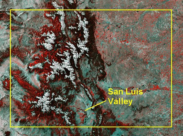
FIGURE 1: Satellite Map of Colorado with the San Luis Valley
The goal of this instructional module is to use a band ratio technique to identify the amount of agricultural land receiving irrigation water in a portion of the San Luis Valley. A Landsat Enhanced Thematic Mapper (ETM+) data set, taken during the late summer (August 26, 2002), is used in this exercise. A subset from this ETM+ data set was formed to create a study area. The study area is 842.7 square miles (2182.6 sq. km) in size and is situated in the northwest section of the Valley, north of the Rio Grande (Figure 2) and around the community of Center.
BACKGROUND:
San Luis Valley
The San Luis Valley is situated in south-central Colorado. It is a large, flat intermountain valley that varies from 40 to 65 miles (64 to 105 km)east to west and is about 100 miles (161 km) north to south in size. The state of Connecticut could easily fit on the valley floor, not including the surrounding mountain slopes. The valley floor rests at about 7600 feet (2316 m)above sea level. Outlining this huge valley are the snow-covered peaks of the Sangre de Cristo Mountains on the east and the San Juan Mountains on the west (Figure 2). The immensity of the Valley with the surrounding mountains provides an outstanding panoramic view. Here supposedly is the highest and largest alpine valley in the world.

FIGURE 2: NASA – MODIS image of the San Luis Valley taken on June 11, 2002
Physical Setting
The San Juan Mountains rise slowly from the valley floor and eventually reach elevations exceeding 12,000 feet (3658 m). By geologic standards these mountains are very young, coming into existence between twenty-two and twenty-eight million years ago. They consist mostly of volcanic rock and provide a rugged landscape. The Sangre de Cristo Mountains ascend dramatically and rapidly from the Valley and attain heights well over 14,000 feet (4267 m). These mountains were formed through faulting, a process where mountains push up abruptly along a fault line system. The mountains are only 10 to 20 miles (16 to 33 km) wide but soar well over a mile above the valley floor. These mountains are slightly younger than the San Juan Mountains with the last significant uplift occurring about twelve million years ago. They provide a sharp contrast to the valley floor. At the north end of the Valley these two mountain ranges bend toward each other and help form the Valley’s elliptical shape. The ranges meet at Poncha Pass, which is the main gateway to the upper Arkansas Valley. The south end of the Valley is not as well defined but the large, rounded volcanic mounds known as Ute Peak and San Antonio Mountain, both located just slightly over the border in New Mexico, provide nice entry points into the Valley.
Out of the San Juan and Sangre de Cristo mountains flow several streams that bring water to the Valley. The largest and best known is the Rio Grande, which starts up in the San Juans and moves initially eastward coming out of the mountains. In the middle of the Valley it turns southward and travels into New Mexico. In addition to the Rio Grande, the Conejos River, Alamosa River, and the Saguache Creek originate in the San Juan Mountains. The Sangre de Cristo Creek, Trinchera Creek, and Culebra Creek are the major streams coming from the Sangre de Cristo Mountains. A great number of smaller, and often intermittent, streams flow from both mountain ranges and provide green riparian sanctuaries across what is a generally brown, arid landscape.
The San Luis Valley is a structural basin where the edges faulted and the mountains on both sides rose and the valley floor dropped. This basin forms the northern portion of a large structural system called the Rio Grande Rift. This rift travels through the center of New Mexico into northern Mexico. During the process of dropping, the valley floor on the east side decreased about 20,000 feet (6096 m) more than the floor on the west side; however, over the years sediment from the adjacent mountains has filled this trough making the floor relatively flat. Along the edge of the mountains, gentle-sloping alluvial fans have formed and have coalesced creating piedmont alluvial plains. These plains allow water to flow gradually toward the center of the Valley.
Climatically the San Luis Valley is a cool desert. Like many deserts it receives a tremendous amount of sunshine in all seasons of the year and has beautiful blue skies during the day and clear star filled skies at night. It receives on the average around eight inches of precipitation per year, but it is not uncommon for it to get twelve inches of snow in a day or experience a sudden downpour of one or more inches of rain. Typical of many deserts the Valley’s weather is one of extremes.
Summer daytime temperatures in the Valley are moderate. They are generally in the mid 70s to low 80s degrees Fahrenheit. With the low humidity these temperatures are very comfortable. Temperatures rarely exceed ninety degrees. The Valley is one of the major potato growing regions within the country and the warm, sunny days and cool nights provide a perfect growing season. The cool weather also contributes to the smoothness of the potato skin. Winter daytime temperatures are temperate with highs being in the 40s to 50s degree Fahrenheitlevel. However, with clear skies and calm winds, nighttime temperatures can reach below –30 degrees Fahrenheit. The Valley will often record the lowest temperature in the nation during the winter. Winter temperature inversion adds to the rawness of the winter weather in the Valley. Cool air from the surrounding mountains can flow down into the Valley on winter evenings. Since the cool air is denser, it settles in the lower elevations unless wind is able to circulate it. Inversion occurs when cold air is trapped on the valley floor by layers of less cold air from the mountains. Under these conditions temperatures will increase as one travels up into the mountains.
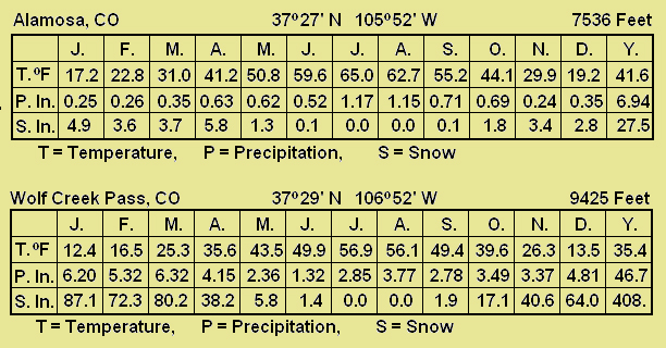
Average precipitation rates vary from seven to ten inches with most of the precipitation occurring in the summer from thunderstorms. See the climatic table for Alamosa, which is located basically in the middle of the Valley. Storms generally do not cover the entire Valley. A person can frequently observe rain occurring in several different places within the Valley but never receive any rain at his/her location. Winter precipitation levels are lower than summer levels with most precipitation being in the form of snow. The Valley falls within the rain shadows of the mountains around it. Storms entering the Sangre de Cristo Mountains generally start over the Gulf of Mexico. They initially cross the humid coastal plain of Texas and then work their way over the plateau edge and hills of central Texas, where they can dump sizeable amounts of rain due to orographic uplift. Once on the high plains of western Texas, these storms do not encounter any major orographic barriers until they reach the Sangre de Cristo Mountains. Since the storms are coming from the east, it is the east side of the mountains that receive the greatest amount of precipitation. These storms have very little moisture left by the time they reach the Valley. Air masses from the Pacific Ocean provide moisture for the San Juan Mountains. Coming from the west, more moisture falls on the west side of these mountains than on the east side. Also, due to the wind patterns associated with these air masses most of the moisture comes during the winter in the form of snow. See the climatic table for Wolf Creek Pass. Wolf Creek Pass is located in the San Juan Mountains and has one of the highest precipitation levels in Colorado. Again, very little moisture is left in the air once a storm enters the Valley.
TABLE 1: Weather Data
Population
The Valley consists of five counties, namely Alamosa, Conejos, Costilla, Rio Grande, and Saguache. Large sections of each of these counties occupy the valley floor where most of the water demand occurs. Also, portions of each of these counties extend to the crest lines of the surrounding mountains. Based on the 2000 U.S. Census, the total population for these five counties is 45,359. Of this number, 27,379 reside in Alamosa and Rio Grande counties. Alamosa County occupies the center of the Valley and contains the city of Alamosa, which is the largest community and the most important central place in the Valley. Population density ranges from 20.81 people per square mile in Alamosa County to 1.86 per square mile in Saguache. These densities are well below the population densities of Colorado and the United States, which are 41.52 and 79.50, respectively.
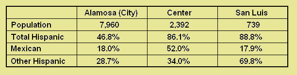
The Hispanic and Latino population makes up 47.16 percent of the Valley’s total population. Individuals from Mexico make up 16.51 percent and a census category of “Other Hispanic” has 30.65 percent of the total population. A large portion of the “Other Hispanic” category consists of people who trace their families back to the 1800s when the Valley was first settled by Europeans and are more likely to view themselves of Spanish heritage. Throughout this module, discussion will relate to the communities of Center and San Luis. It might help to look at their Hispanic character. As indicated in the table below the vast majority of the people who reside in Center and San Luis are Hispanic. In the city of Alamosa, the Hispanic population is slightly less than half. In both Colorado and the United States, the percent of Hispanic population is 12.5. The major difference between Center and San Luis is that slightly over half of Center’s total population is Mexican and nearly 70 percent of San Luis is Other Hispanic. Center’s Mexican population works mainly on the large center pivot irrigation farms that are owned by wealthy farmers living in the city of Alamosa. San Luis’ "Other Hispanic" population are farmers who have small, long-narrow farms that have been in their families for generations.
TABLE 2: Hispanic Population Data for Selected Communities
Aquifers
Much of the water received by the Valley comes from the surrounding mountains but a great deal of the water is not at the surface level. As the water leaves the mountains large amounts of it penetrates the ground at the edge of the Valley and seeps into aquifers. The aquifers contain an estimated two billion acre-feet of water and whatever water is removed from them is easily replenished. Two basic types of aquifers exist within the Valley. The first are referred to as unconfined aquifers. Water in such aquifers is very near the ground surface and flows freely through the loose mineral material of the aquifers. Since the water is near the surface, little water pressure exists in the aquifer. These aquifers are generally recharged from precipitation, streams, and canals. Within the Valley unconfined aquifers are found less than twelve feet from the ground surface and can be easily tapped by wells.
The second type of aquifer exists when a permeable layer in the ground is enclosed above and below by impermeable layers as illustrated by Figure 3. This is a confined aquifer. As water accumulates in a confined aquifer, water pressure builds until breaks occur in the impermeable layers creating artesian seepage. The first drilled artesian well in the Valley occurred in 1887 and within ten years, over 3,000 wells existed. Confined aquifers are found in the upper 6,000 feet of the Valley sediment, making them much deeper than unconfined aquifers. Artesian wells in the Valley only have to be drilled between 100 and 200 feet in order to obtain enough water. Due to the abundance of water most artesian wells were not capped until the 1960s when farmers were finally ordered to stop wasting the water. Prior to the 1960s the free-flowing wells produced large ice sculptures during the winter months by shooting water into the air where it would freeze. Eventually, these huge sculptures would cap the wells. Confined aquifers have played a key role in the development of central pivot irrigation in the valley.
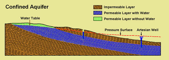
FIGURE 3: A cross-section of a confined aquifer
Hot springs occur along the eastern and northeastern sides of the Valley. These springs are natural artesian wells that have been heated deep within the earth. One well receives water from 2050 feet deep and discharges water continuously at 87° F (30.5° C). In 1977, a tilapia farm was established around the well. Native to Israel and Africa, tilapias are warm-water fish raised for food. This venture became an economic success but several thousand pounds of filleted fish carcasses, dead tilapia, and trash fish were being generated each year. To overcome this problem, American alligators were introduced. Today, the farm supports a sizeable alligator population, which has become a tourist attraction. It is something to observe 10 foot, 500 pound alligators resting in snow around the edge of hot springs. One would not expect to find an alligator ranch in the middle of the arid American West but this situation does illustrate what can happen as a result of man using water under the right conditions.
Water Rights
In the more humid, eastern half of the United States, the riparian doctrine, obtained from the English, gives landowners the right to use any water on their property. Under these rights water naturally flowing on a person’s property cannot be diminished. The abundance of water generally permits it to be shared equally by all users. However, in most of the western half of the United States, water is a precious resource that needs to be appropriated. People in the West have to deal with the law of prior appropriation. The first person to put a water source to “beneficial use” has the first right to water from that source when water is scarce. A water right is a property right, which is not connected to the land on which the water occurs. A water right can be transferred to a farmer or city miles away from where it exists. However, the transfer of water is highly regulated. In Colorado, the state engineer and the seven water courts throughout the state oversee the transfer of water.
Early Water History
In the 1600s the Spanish started establishing settlements in what is today northern New Mexico. Although they had visited and claimed the San Luis Valley, it was not until the mid-1800s that they tried to develop settlements within the Valley. Apparently, they did not want to move north of Taos, New Mexico in order to placate the Ute who considered the mountain regions of Colorado their homeland. In 1821, Mexico gained independence from Spain and wanted to inhibit any encroachment by the United States or the new Republic of Texas on its northern territories. Following the same approach that the Spanish had used throughout the Southwest, the Mexican government made several large land grants to individuals who would colonize the Valley. Figure 4 shows the major land grants in Colorado. Only three of these grants (Conejos Grant, Luis Maria Baca Grant, and Sangre de Cristo Grant) relate to the Valley. During the 1840s, the grantees attempted several times to establish permanent settlements on their land but the Indian threat kept them from achieving their goal. This condition continued until the end of the Mexican War in 1846, after which the United States military forces made a concerted effort to remove the Indian problem. Encouraged by these events, the first successful settlements occurred in the 1850s. The town of San Luis was established in 1851 on the Sangre de Cristo Grant and has the distinction of being the oldest town in Colorado.
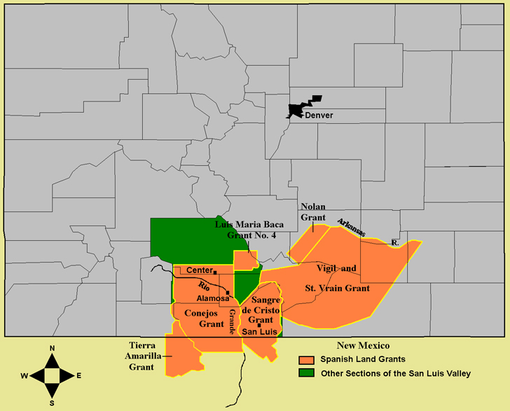
FIGURE 4: Spanish Land Grants in Colorado
Following the traditional Spanish settlement patterns, these early communities developed around central plazas. Homes were built around the plazas and farmers would go out to their fields to work. These homes, constructed of adobe materials had no windows and the doors opened out onto the plaza. This layout allowed the communities to protect themselves from Indian attacks. After a community was established, the next task was to dig an irrigation ditch, called an acequia. The irrigation ditch in San Luis has the first recorded water rights in Colorado. Within a few years, forty of these ditches were built throughout the southern portion of the Valley. These ditches are designed to work on the gravity system, where water taken from them would flow to fields located at lower levels. Initially, the water would be hauled out of the ditches and dumped into fields but today it is siphoned out. Long, narrow strips of land were laid out along these ditches in order to provide each farmer access to the irrigation water and the same ecological zones back from the ditch. These long strips of land are called vara strips. (A vara strip is named after the Spanish the linear measurement unit, vara, which is 32.909 inches or 2.78 feet. A vara strip is a certain number of varas wide. ) Not all sections of these lands could be irrigated. A public pasture next to the community, called a vega, was established. Centered on their irrigation ditches the people in these communities led a pastoral life based on farming and sheep herding, a pattern that still exists today in many areas of the Valley.
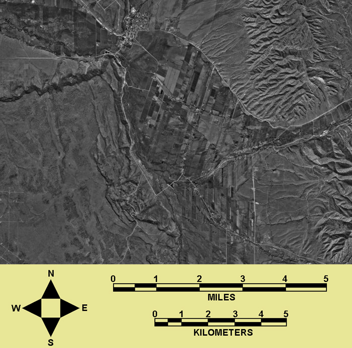
FIGURE 5: San Luis and vara strips in the Culebra Creek Valley (Photo Taken: Sept. 29, 1999).
Figure 5 shows the town of San Luis, which is located near the upper edge of the aerial photograph. The photograph also shows the long, narrow irrigated fields in the Culebra Creek Valley and how they stand in contrast to the drier, non-irrigated land surrounding the valley. The land in the valley is gradually sloping downward toward the northwest. Culebra Creek runs along the western edge of the valley. The irrigation ditches tap the creek farther up the valley and flow through the center and on the east side of the valley. By gravity the water in these ditches flows northwest. Farmers direct the water from these ditches into their fields using the siphon tube method. The individual fields are small in comparison to the large center pivot fields in other sections of the San Luis Valley. Crops tend to be vegetables that meet the needs of the local market such as beans, lettuce, spinach, corn and peppers. The long lot pattern stops before reaching the community of San Luis. The large section of land just south of the community is the 633.32 acre common grazing land, which has lush, irrigated grass. Hard to detect on the photograph are the very small communities of San Pedro, San Pablo, Chama, and Los Fuertes. They are called the villages of the Rio Culebra. Established at the same period as San Luis, they were farther up the Culebra Valley and away from where the Culebra Creek cuts through the San Pedro Mesa. San Luis is located at the gap in the mesa where the creek flows and is at a key transportation and water flow point. Reflecting the community’s strong and continuing Spanish heritage is the Chapel of All Saints, La Capilla de Todo los Santos, which was completed in 1996 and located on the mesa above San Luis. With its domes, portal, and ornamental arabesque windows, and with its bright white exterior seen from miles away, it is a clear linkage to the Islamic-Spanish landscape.
In 1861, the Territory of Colorado was established, which resulted in the Valley being no longer part of the New Mexico territory. Politically and economically this change separated the Hispanic settlements in the southern portion of the Valley from their traditional base. After nearly two hundred years of being isolated from Spain and Mexico, the people of the Rio Grande region of northern New Mexico and southern Colorado were strongly linked by their archaic Castilian Spanish language. Even today these people, based on their language and traditions, remain very conservative and cut off from the main growth within the Valley. Costilla and Conejos counties, the two southernmost counties in the Valley, are among the poorest counties in the country, mainly due to this isolation.
With the passage of the Homestead Act of 1862 and the end of the Civil War in 1865, Anglo settlers entered the Valley in large numbers, especially in the northern sections of the Valley. They found the non-Spanish grant sections of the Valley laid out in the Public Land Survey systems, something that they were familiar with from the Mid-West and Great Plains areas of the country. By 1866, the land around Saguache was being heavily homesteaded and was separated from Costilla County to become a new county. In 1874, Rio Grande County was separated from Conejos County. With the arrival of the Denver and Rio Grande Railroad, the town of Alamosa was laid out in 1878. The railroad brought the necessary transportation to establish commercial agriculture in the Valley. During this period, DeWitt C. Travis, the first commercial potato grower in the Valley, was producing 70,000 pounds of potatoes per year. Alamosa County was created in 1913. These developments divided the Valley geographically between the old Hispanic way of life and the new Anglo settlements, and more importantly, in the use of water.
During the 1880s several canal systems were founded throughout the Valley. Started in 1881 the largest of these systems was the Rio Grande Canal. This system consists of 210 miles of canals and laterals and 517 individual farm headgates. It furnishes water to 120,000 acres of land in Alamosa, Rio Grande, and Saguaches counties. Completed in 1884, the canal’s main channel is sixty feet wide at the bottom, ninety feet wide at the top, five feet deep at the sides, and six feet deep in the middle. For the time period, the construction of this system was a major engineering accomplishment and a clear indication as to how water was going to be handled in the Valley under Anglo development. Today, thirty-one prior appropriations take 1699 cubic feet per second of water from the canal. In an average year thirty percent of the Rio Grande water is diverted into this canal system.
Water Problems
By the 1880s water conflicts were occurring and the need arose to adjudicate water rights. In 1888, a General Adjudication of water rights occurred with supplements being added over the years. In addition to water conflicts, a severe drought hit the Valley and other areas in 1893, resulting in bank failures, farmers leaving the Valley, and some small communities disappearing. The Rio Grande dried up along the Texas-Mexican border. By 1896, the situation had changed and a water surplus existed. In the Mosca and Hooper areas the water table was seeping through the valley floor due to poor irrigation procedures associated with a high water table and no natural drainage. The procedure involved forcing the water table in the unconfined aquifers to rise to a level where the roots of crops would be saturated. The problem with this method was that it also drew salt, which in turn, ruined the soil. Fields were abandoned but the water continued to rise to the surface where evaporation of the standing water resulted in more salt or alkali conditions. Topographically this area is an enclosed basin with no drainage. By the 1920s many acres had become waterlogged and/or alkalined, and had been taken over with greasewood and rabbit brush. This condition still exists today around Mosca and Hooper.
The water shortages and soil problems of the 1890s reached beyond the Valley. Increased farming in the Valley had resulted in less water for farmers in New Mexico and beyond. By the time the 1893 drought occurred, the Rio Grande riverbed at El Paso was dry. In the Valley all of the canals except the Rio Grande Canal were empty. The Rio Grande Canal was using all of the water in the Rio Grande to deal with the earliest of prior appropriations. Later appropriations were receiving no water. In 1896, an International Boundary Commission was established for the purpose of developing a plan where water would be equitably distributed between Colorado, New Mexico, Texas, and the Republic of Mexico. Even though Colorado controlled the headwaters of the Rio Grande, an embargo on developing any water diversion projects on the upper Rio Grande occurred until 1906. The people in the Valley were discovering that they had to share the Rio Grande water. A treaty was signed in 1906 by the United States and Mexico that allowed Mexico to receive 60,000 acre-feet of water every year. To fulfill this commitment, the Elephant Butte Reservoir was built on the Rio Grande in southern New Mexico in 1916. This reservoir has a storage capacity of 2,600,000 acre-feet.
Center Pivot Irrigation
Surface flood irrigation was the primary method of distributing water to the field during the period from the 1890s to the early 1960s. Large siphon tubes were used to draw water from the irrigation ditches into the fields. Basically it was the same method that the Hispanic communities used with their acequiaes but on a much larger scale. In the 1960s, center pivot sprinkler systems (Figure 6) started to replace most of the surface flood irrigation by tapping the tremendous amount of water available in the confined aquifers. These aquifers had been tapped in the late 1800s through drilled artesian wells. The water from these wells was used for surface flood irrigation.
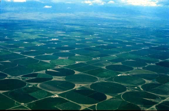
FIGURE 6: An oblique aerial photograph showing center pivot fields in the San Luis Valley.
The center pivot system provided a new method for irrigating fields. This system is based on a well being in the center of a field and an irrigation pipe mounted on wheels gradually moving around the well. This arrangement forms circular field patterns. Most of the center pivot systems are found in the northwest portion of the Valley, mainly in Saguache, Rio Grande, and Alamosa counties. These counties were organized under the Public Land Survey system with the basic land parcel being the quarter section. A quarter section covers 160 acres. Since the initial center pivot systems were designed chiefly for quarter section land parcels on the Great Plains, it was relatively easy to apply the technology to similar areas under the Public Land Survey system. An examination of Figure 7, a mosaic of aerial photographs taken over the northwest portion of the Valley, shows how the circular fields are arranged in the neat grid pattern associated with the Public Land Survey. Each circle rests inside a 160-acre quarter section. Figure 2, a satellite image covering the entire Valley and surrounding mountains, illustrates how the center pivot system is mainly concentrated in the northwest section of the Valley with smaller, isolated clusters scattered throughout other areas of the Valley. The crops grown in these fields are mainly potatoes and alfalfa with some lettuce and spinach as secondary crops. Potatoes, lettuce, and spinach are produced for the national market. Alfalfa is grown for the dairy farms in New Mexico and Texas. Some fields are owned by Coors for the production of barley.
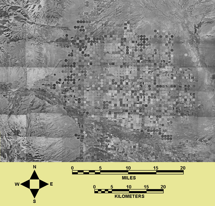
FIGURE 7: Center pivot fields in the Valley (Photo Mosaic: Sept. 6, 1998).
Initially, the sprinklers on the irrigation pipes shot water up into the air in a whirling motion spraying large areas (Figure 8) but it was discovered that large amounts of the water was lost due to evaporation. Today, lines drop down from the irrigation pipe to within a foot or two of the plants and spray immediately above the plants. This drop line method significantly reduces the amount of water needed. Also, water to these lines is highly computerized. If the drop line sprinklers near the center of the field were permitted to distribute the same amount of water as the sprinklers on the edge of the field, the center of the field would be flooded. Such flooding would be a waste of water and could result in the alkalization of the center of the field.
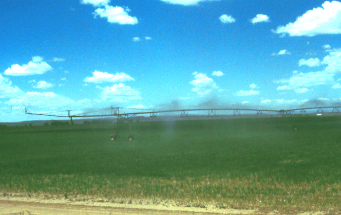
FIGURE 8: Center pivot irrigation pipe spraying water on an alfalfa field.
Figure 9 shows the high concentration of center pivot fields around Center, Colorado. Some of the fields are not absolute circles. On the sides of the fields the edge of the circles are truncated. In many cases what the farmer is doing is allowing water to shoot out at the end of the irrigation pipe. This action results in water being sprayed into adjacent fields and the roads separating the fields. It also permits water to reach more into the corner of the fields and use more of the land for production. This approach wastes water and the farmer could be heavily fined for creating dangerous road conditions. A few of the irrigated fields are almost rectangular in shape. Buried around the edge of these fields, at about four feet down, are sensor wires. These wires are used to control the speed of the last section of the irrigation pipe. Rather than the entire length of the pipe being straight, the last section is at an angle when the pipe moves along the edges of the field and then the last section straightens out when the pipe goes into the corners. The last section is frequently referred as the “tail dragger.” This approach represents the best use of the field space, and since only drop line spraying is required, it also represents the best use of the water.
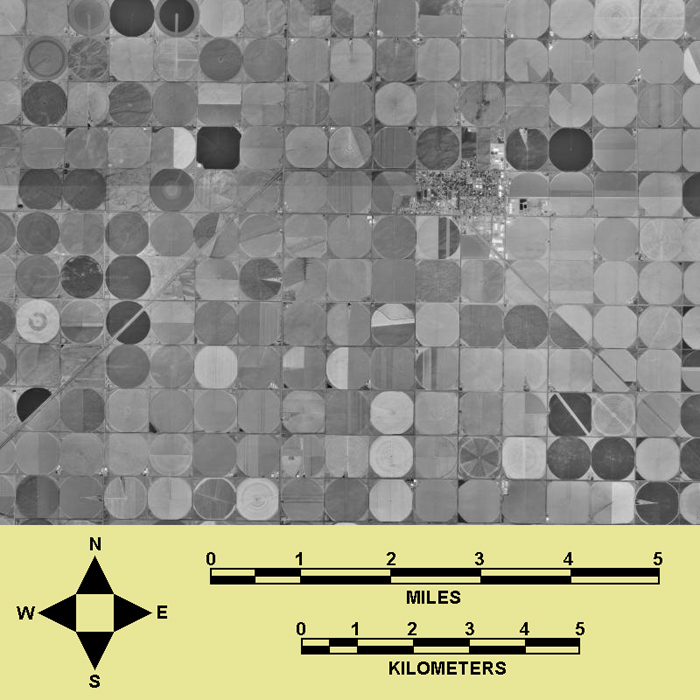
FIGURE 9: Center pivot fields and Center (Photo Taken: Sept. 6, 1998).
The fields shown in Figure 9 offer a variety of patterns. In some cases the farmer has elected to have two different crops in a field. Since the photograph was taken in September, many of the fields are being harvested and farmers experiment with different ways of harvesting circular fields with respect to energy use on their equipment. Some narrow straight lines can be detected in some of the fields. Frequently these are service roads that allow farmers access to a well and pump. The two long diagonal lines are irrigation ditches. They are cutting diagonally through some fields. Some of the farmers who have these fields have two center pivot irrigation systems, one on each side of the ditch. Other farmers have put small bridges across the ditches to accommodate the wheels of the irrigation pipe. When the pipes cross over the ditches using these bridges the drop line sprinklers are programmed to stop working and then start up again once across a ditch.
Two major problems exist in using center pivot irrigation in the Valley. First, the water from the confined aquifers brings to the surface large amounts of salts. When the water evaporates on the surface or evapotranspires through the plants, salt is left behind in the soil. If the salt is allowed to build up, it can destroy the capability of the soil. Excess water must be used on the fields to break up the salt and carry it back below the ground level. The second problem relates to energy costs. To pump large amounts of water over long periods of time and to move large irrigation pipes around the field takes a tremendous amount of energy. Since energy prices fluctuate, a farmer finds it difficult to judge energy costs, which is a major item in the overall production of a crop.
Closed Basin Project
As the Rio Grande flowed out of the San Juan Mountains and into the center of the Valley, it carried a tremendous amount of sediment, which eventually formed a barrier to the flow of streams coming from the northern section of the Valley. Essentially, a closed basin was created with internal drainage. This condition resulted in the water from the unconfined aquifer rising very near the surface, and in some cases, seeping onto the surface. Water was lost to evaporation and alkali formed in the fields.
The national and international water agreement of 1939, called the Rio Grande Compact, required Colorado to transfer more water downstream to New Mexico, Texas, and Mexico. Too much water was being taken from the Rio Grande by the Valley for agricultural development and not enough was being sent downstream. Of course, center pivot irrigation based on confined aquifers had not yet been developed and about thirty percent of the Rio Grande water was being diverted into canals in the Valley. Initially envisioned in the 1930s, the Closed Basin Project did not get started until the 1980s. Under this project, 170 wells are tapping water in the unconfined aquifer in the closed basin and pumping 100,000 acre-feet of water per year into an aqueduct that transfers the water to the Rio Grande for use downstream. This project is also lowering the water table in the unconfined aquifer by two feet per year and reducing alkalization. Today, Colorado is over-delivering water to the state line and has established a credit that will assist the Valley in dry years. However, the removal of water from the Valley’s aquifers to meet outside needs might have opened the door to other demands.
The Baca Project (AWDI)
In 1986, the American Water Development, Inc. (AWDI) was formed and filed an application in a water court to remove 200,000 acre-feet of water per year from 112 proposed wells on the Luis Maria Baca Grant land. This water was to be shipped to the growing urban areas along the Front Range of Colorado. Boulder, Denver, Colorado Springs, and other Front Range cities are finding it difficult to obtain enough water to meet their present growth conditions let alone any future growth. This well-financed and well-organized project approached the extraction of the water as a mining endeavor. AWDI argued that the removal of this amount of water would not impact other water users in the Valley. Farmers, ranchers, and several state and federal agencies fought this project and bitter and extensive litigation lasted several years. AWDI lost the case and their subsequent appeals all the way up to the U.S. Supreme Count. It had to pay $3.0 million to the organizations legally objecting the extraction of the water. In 1995, AWDI sold the Baca Grant property. Although it won this case the Valley needs to be prepared for other challenges to remove its water. The conflict between urban and rural demands for water in the arid and semiarid regions of western United States is likely to become more intense in the future as the country’s population grows and shifts westward.
ANALYSIS:
As stated previously a subset from the Landsat ETM+ data set (August 26, 2002) was developed for this exercise. This subset is 1590 lines by 1690 picture elements (pixels) in size and each pixel covers a ground area of 28.5 m by 28.5 m. This subset corresponds to the large center pivot irrigation area located in the northwest section of the Valley, mainly north of the Rio Grande (Figure 10). In the middle of the study area is the community of Center, which is at the lowest spot within the Closed Basin. The San Luis Valley experienced a five year drought from 1999 to 2004; thus, the data set was collected in the middle of this drought. Because of the large number of center pivot irrigation fields surrounded by dry land this subset makes for an ideal study area to determine if agricultural land receiving irrigation water can be separated from other land cover, and if the amount of land, covered by irrigation water can be measured.
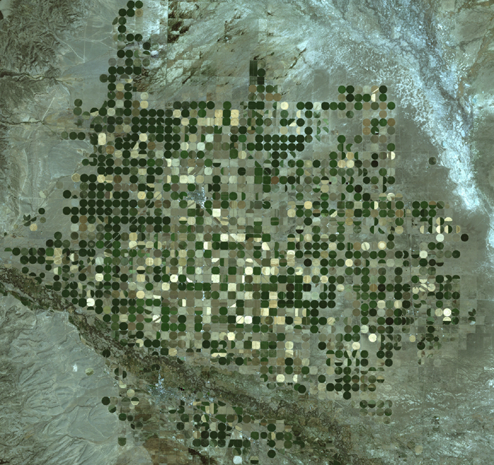
FIGURE 10: True color image of the study area.
As the Background section of this module tried to illustrate, water issues in dry regions are complex and are intertwined with cultural, economic, and political expectations and technological abilities. Within this context, this exercise deals with identifying those center pivot irrigation fields within the study area that are being irrigated. Center pivot irrigation has become a widely used means of irrigation not only in western United States, but also in many dry regions throughout the World. The San Luis Valley was selected for this exercise because of its high usage of center pivot irrigation, its strong emphasis on agriculture in its overall economy, and its cultural differences pertaining to irrigation.
A regular ETM+ data set has nine spectral bands. Bands 1-5, 7 measure reflective energy in different portions of the electromagnetic spectrum and have a pixel resolution of 28.5 m by 28.5 m. Bands 1-3 relate to the visible range of the spectrum; whereas, Band 4 deals with the near-infrared and Bands 5 and 7 with two diffenet portions of the mid-infrared. Bands 61 and 62 record emitted energy in the thermal infrared portion of the spectrum and have a resolution of 57 m by 57 m. Band 8 covers a wide section of the spectrum and has a resolution of 14.25 m by 14.25 m. Bands 1-5, 7 are provided with the subset. This exercise is based on using only Bands 4 and 5. The software package, EarthScenes, is used throughout this module and all the functions required to complete the tasks associated with this exercise are available with this package.
Band Ratioing
Band ratioing provides a way to generate new images that can assist in detecting certain environmental conditions, especially with respect to vegetation coverage. Active vegetation strongly absorbs red light in the visible portion of the spectrum and strongly reflects near-infrared (NIR) energy. No other major Earth surface materials demonstrate these spectral conditions. Research has also determined that mid-infrared (MIR) bands depict the moisture content of active leaves. Based on this information, many mathematical Red-NIR-MIR combinations have been developed as vegetation indices. The table below provides some of the more applied vegetation indices.
TABLE 3: Vegetation Indices
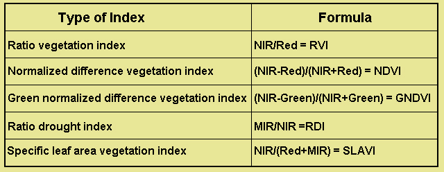
The Ratio Vegetation Index (RVI), also referred to as simply the Vegetation Index (VI), divides the red visible band into the near infrared band. For Landsat, MSS bands 4/2, and TM and ETM+ bands 4/3 are used. The most mentioned index is the Normalized Difference Vegetation Index (NDVI). This index has been heavily applied to global vegetation patterns using NOAA’s Advanced Very High Resolution Radiometer (AVHRR) sensor system. It has also been frequently used with Landsat data. Less used is the Green Normalized Difference Vegetation Index (GNDVI). It employs the same formula as the NDVI but in place of the red visible band, it uses the green visible band. The Ratio Drought Index (RDI) is designed to detect vegetation experiencing drought conditions and with little moisture content. It is this index that will be used in this module. The Specific Leaf Area Vegetation Index (SLAVI) attempts to measure the functional health and productivity of certain forest, rangeland, and crop conditions.
As can be seen by the various formulas, the creating of vegetation indices involves using one or more mathematical operations on two or more integer based data layers (bands). Such operations result in output of fractional real numbers. These real numbers create a problem for a database designed to deal with integer values. More specifically, Landsat databases deal with only integer values between 0 and 255, the range of a compute byte. When first calculated, NDVI values can range from +1 (maximum vegetation) to -1 (no vegetation). To convert these values so that they relate to the byte format, the standard conversion formula ((NDVI+1) x 100) is used. This operation results in values ranging from 0 to 200, that relate well to the byte format. It also allows the index values to be used in conjunction with the spectral band values in the database to develop other products such as false-color images
Procedures
As previously indicated, Bands 1-5 and 7 form the data set for this exercise. Load Bands 4 and 5 into EarthScenes. The exercise only requires these two bands; however, one might wish to load all six bands in order to observe what information the other bands might provide for this type of environment.
Create histograms for both Bands 4 and 5, and then, plot the histograms for the purpose to see how the data are distributed across the spectral range of 1 to 250. Note that Band 4 has a minimum value of 1 and maximum value of 190. However, the histogram plot shows that most of the data falls into a smaller range. In fact, 99.9 percent of all the data is between 40 and 178. Using this information, contrast stretch Band 4. Make a new layer for the stretched band, and name it, “Band 4 Stretched 40 to 178.” Assign 40 as the new minimum value and 178 as the new maximum value. In the contrast stretching process, values from 1 to 40 will be given the value of 1 and values from 178 to 190 will be assigned to 250. All values between 41 and 177 will be proportionally given values between 2 and 249.
Repeat the process described above for Band 5. The minimum and maximum values for Bands 5 are 1 and 250. However, the histogram plot shows that 99.9 percent of the values are between 41 and 230. Using these values, contrast stretch Band 5. Make a new layer for the stretched band and name it appropriately. Figure 11 shows four sub-images of the same portion of the study area. The upper left sub-image of the picture contains the original Band 4; whereas, the upper right sub-image has the stretched Band 4. The same arrangement applies for Band 5, except that the original is in the lower left and the stretched version in the lower right. By comparing an original image to a stretched image, one can gain an understanding how contrast stretching can enhance an image.
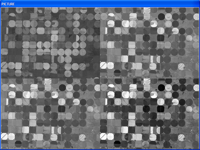
FIGURE 11: Original and stretched band comparison.
As indicated in the section on band ratioing, the Ratio Drought Index formula will be used in this exercise. This formula deals with dividing stretched Bands 5 and 4 (5/4) to create a drought index layer. EarthScenes has an arithmetic operation section that allows mathematical procedures to be performed on two layers. Select option 6 under this section, which allows one layer to be divided into another layer. Name the new layer, “Drought Index.” Create a histogram for this new layer and plot the histogram. The histogram shows that the index data are scattered over the entire data range. Thus, it is not necessary to contrast stretch this layer.
Create a false color composite assigning the Drought Index to the red layer, the stretched Band 5 to the green layer, and the stretched Band 4 to the blue layer (Figure 12). This composite shows vegetation with little moisture content as being in red and reddish orange. This is the influence of the Drought Index on the composite. Large areas outside the center pivot irrigation fields fall within these red colors. These areas are covered by dry land vegetation. The bright and dark blue areas, mainly associated with the center pivot irrigation fields, have vegetation with high moisture content. This is the result of the Drought Index having very low values in these areas and the near-infrared (Band 4) having strong reflectance values from green vegetation.
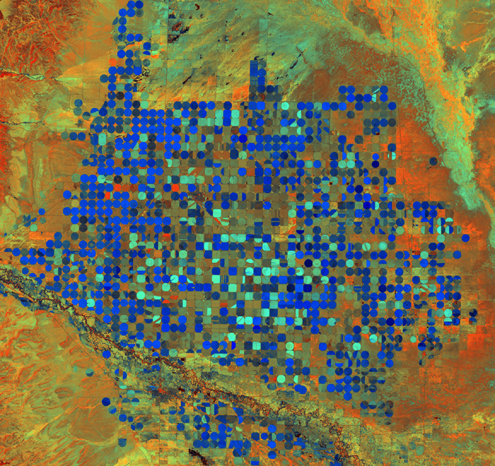
FIGURE 12: False color composite of the study area.
The next step is to conduct a density slice classification of the Drought Index layer. Since the objective of the exercise is to separate agricultural land being irrigated from other land cover and measure the amount of land covered by irrigation water, the classification should consists of two classes. One class should identify vegetation with high moisture content and the other class should cover everything else. In order to determine the density class range for the first class, use the pixel read-out function on the false color composite just created. Move the cursor over the blue-colored fields and note the values being displayed under the red level. These values will generally range from 1 to 20. They indicate a low drought condition, meaning moist vegetation. Now plot the histogram for the Drought Index layer. Note the high points and low points on the histogram. The range from 1 to 20 relates to one of the high points but to separate this high point from the next high point, one needs to select a value from the low point between the two high points. The lowest value between the two high points is 37. Thus, the range for the first class will be 1-37 and for the second class it will be 38-250. Figure 13 illustrates the two classes. The red and green colors on Figure 13 are generated by the density slice classification function. Save the classification as a new layer. One might want to define the two classes in a different manner, and thereby, create different classification results
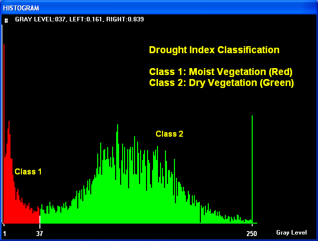
FIGURE 13: Density slice classification of dorught index layer.
The new classification layer contains only values of “1s” and “2s” to correspond to the two classes. When the classification layer is being created, a count as to how many pixels are associated with each class is maintained. This information should be recorded in order to be used later to measure the amount of land in each class. In this case, class 1 has 434,192 pixels and class 2 has 2,252,908 pixels.
The next step is to reverse the two classification numbers in order to highlight the moist vegetation class. This reversal process can be accomplished by getting the reciprocal values of the numbers. Under this process the classification numbers are divided into the constant of 1. EarthScenes does not provide a direct way to generate reciprocals. Thus, a layer that contains only “1s” must be first produced. Select any band that has a generated histogram and do a single class density slice classification on it. This will produce a new layer where all of the pixels have values of “1.” The Drought Index classification layer is divided into this new classification layer using option 6 under the arithmetic operations provided by EarthScenes. Make sure to scale the output into the range of 1 to 250. Once completed, the classification values for the second class now have a value of "1" and the classification values for the first class, the moist vegetation class, have a value of "250." Name this new layer, “Reversed Drought Index.”
With a value of 250, the pixels related to the moist vegetation class can be highlighted when displayed. To illustrate this situation, add the original Band 5 and the Reversed Drought Index layer together to create a new Band 5 layer. Use arithmetic option 4 with a constant of 1 to do this addition. Truncate the output at 1 and 250. Once the layer is generated, create a false color composite using the original Band 5 layer for both the red and green colors and the new Band 5 layer for the blue color (Figure 14).
The blue color on Figure 14 relates to areas with moist vegetation coverage. In other words, these areas are not experiencing drought conditions. With few minor exceptions the blue colored areas correspond to center pivot irrigation fields. However, not all fields are blue. Most likely, these fields have been harvested and they are not being irrigated. A few blue colored areas exist along the Rio Grande, which are wetlands adjacent to the river. The few, elongated blue colored areas at the top of Figure 14 relate to vegetation conditions where water is seeping from unconfined aquifers in the Closed Basin.
Previously, the number of pixels associated with the two classes was determined after the density slice classification was executed. The numbers were: 434,192 (class 1) and 2,252,908 (class 2). A pixel covers a ground surface of 28.5 m by 28.5 m or 812.25 square meters (8742.9 sq. ft.) . Multiply 812.25 times 434,192 (number of pixels) to determine the number of square meters (352,672,452) related to moist vegetation. A hectare is equal to 10,000 square meters; thus, divide 10,000 into 352,672,452, which provides the number of hectares for class 1. To convert this number into square kilometers divide 100 into the number of hectares. See Table 4 for results.
TABLE 4: Classification reults.
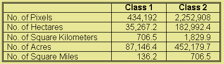
To ascertain the number acres and square miles, first multiply 8742.9 by the number of pixels for the class, and then, divide by the number, 43,560, which is the number of square feet in an acre. To determine the number of square miles, divide 640, the number of acres in a square mile, into the number of square feet in an acre.
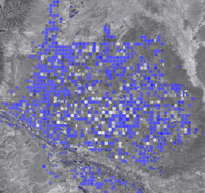
FIGURE 14: Gray level image with moist vegetation in blue.
FINAL COMMENTS:
This exercise started with the statement that, “Water is one of the most precious items on the face of the Earth.” This condition is especially true in the dry land regions where people are generally faced with making the best use of every drop of water. As seen through this exercise, remotely sensed imagery can assist in identifying where water is being used in the agricultural landscape and amount of area being irrigated. It was determined that approximately 87,000 acres or 136 square miles of land was being irrigated within the study area when the imagery was recorded. Nearly all of this land was being irrigated through center pivot irrigation. Generally, a coverage of between 14 and 16 inches of water is sprayed on a field during the growth of a crop. For a typical 127 acre center pivot irrigation field this amount of coverage represents about 159 acre feet of water. For 87,000 acres of irrigated land, the amount of water used is approximately 109,000 acre feet. Another way of viewing these figures is to think of a water body that is one foot deep and 13 miles long on each side. Thus, knowing the amount of land being irrigated along with the amount of water being used on a field it is possible to calculate the approximate amount of water being used to grow a crop. Before the use of remotely sensed imagery it was very difficult to determine how much land was being irrigated. Remote sensing can be employed to ascertain how much water is being used to grow crops in dry land areas.
Suggested Books:
Huber, Thomas and Robert Larkin, 1996, The San Luis Valley of Colorado: A Geographical Sketch, Colorado Springs, Colorado: The Hulbert Center Press of the Colorado College.
Ogburn, Robert W., 1996, “A History of the Development of San Luis Valley Water.” The San Luis Valley Historian, 28: 5-40.
Simmons, Virginia McConnell, 1999, The San Luis Valley: Land of the Six Armed Cross, 2nd Edition. Niwot, Colorado: University Press of Colorado.