DROUGHT IN THE COLORADO RIVER BASIN:SHRINKAGE OF LAKE POWELL
COPYRIGHT © 2001 Paul R. Baumann
INTRODUCTION:
Created in 1963 with the completion of the Glen Canyon Dam, Lake Powell became the second largest reservoir in the United States following Lake Mead. Construction on Glen Canyon Dam was started in 1956 and completed seven years later in 1963, after which the water from the Colorado River proceeded to backup behind the dam to form the lake. In June 1980, after seventeen years, Lake Powell reached full pool size with a volume of 27 million acre-feet (MAF) and a surface area of 266 square miles (689 sq. km.).( An acre-foot is roughly 326,000 gallons of water, enough to supply an average family of four for a year.) At full size the reservoir is nearly 186 miles (299 km.) in length with a water depth of 560 feet (170.7 m) at the dam.
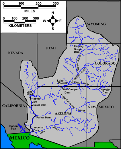
FIGURE 1: Colorado River Basin.
With Lake Powell being located in an arid and semiarid region its water level varies considerably and provides a good barometer of water conditions within the Colorado River’s 246,000 square mile (637,137 sq. km.) basin (Figure 1). From 1995 through 1999 its water level was above average and as late as September 1999, the reservoir was still 95 percent full. However, precipitation levels in the upper Colorado River basin from October through December 1999 fell to 70 percent below average, signaling a low runoff for 2000 and the beginning of an extreme drought.
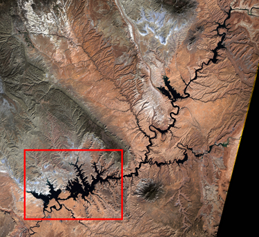
FIGURE 2: Lake Powell – Study Area Outlined in Red.
The goal of this instructional module is to measure the impact of the drought on the lower portion of Lake Powell between 1999 and 2002. The objective is to determine the surface area of the lower portion of the reservoir when the drought started and the amount of change in the surface conditions of the reservoir four years into the drought. Two Landsat Enhanced Thematic Mapper (ETM+) data sets, one taken at the beginning of the drought (October 10, 1999) and the other four years into the drought (June 13, 2002), are used in this exercise. Subsets from these ETM+ data sets were formed to create a study area, the lower portion of Lake Powell. The study area is 676.8 square miles (1089.41 sq. km) in size (Figure 2).
BACKGROUND:
Colorado River Compact
Lake Powell came into existence as part of a larger project to control flooding on the Colorado River and provide water and electrical power throughout the southwest United States. Between 1905 and 1907, several large floods on the Colorado River destroyed crops and fields in southern California, mainly in the Imperial Valley. Floodwaters from the river broke through the irrigation floodgates and flowed into the valley forming the Salton Sea, a 450 square mile (1165.5 sq. km.) lake. From these disasters the idea of building dams to control the river and use its water to meet the growing needs of the dry West was formed. By obtaining money from western land sales and irrigation water the Newlands Reclamation Act of 1902 provided the financial means to build these dams.
In 1922, the Colorado River Compact was established to control the river, and in the process, divided the river into the Lower Basin (Arizona, Nevada, and California) and the Upper Basin (Utah, Colorado, Wyoming, and New Mexico). See Figure 1. Shortly after the compact was formulized, dam construction in the Lower Basin started. Completed in 1936, Hoover Dam was built to regulate flooding and erosion and provide a dependable water supply and hydroelectric power. Downriver from Hoover Dam, the Davis, Parker, and Imperial dams were built to assist in controlling floods. As part of the compact agreement the Upper Basin had to provide the Lower Basin each year with 7.5 MAF of water. In addition, the 1944 Mexican Water Treaty required the United States to release to Mexico annually .73 MAF of Colorado River water, later increased to 1.5 MAF. This water also had to come from the Upper Basin.
Because moisture conditions within the Upper Basin varied greatly from one year to another, the Upper Basin states frequently found it difficult to supply the annual 9.0 MAF of water. To alleviate this situation the U.S. Congress passed in 1956 a bill to build several dams in the Upper Basin. The largest of these dams was the Glen Canyon Dam. Two more large dams, built farther upriver, were the Flaming Gorge Dam on the Green River and the Navajo Dam on the San Juan River. Both of these dams are in headwater sections of the Colorado River Basin.
Today, with a dam almost every hundred miles, the Colorado River is the most dammed river in the United States, which results in it no longer providing water to the Gulf of California. Except in very wet years, the river’s delta is a desert, and what water does reach the area simply disappears into the ground in northern Mexico.
In addition to controlling the river the compact was also established to make sure that each state within the Colorado River Basin received a fair share of the river’s water. In the early 1920s the states within the basin were concerned about California’s growth, and thereby, its increasing consumption and appropriation of the water within the river. This concern was further exacerbated by the fact that California contributed little water to the river. This concern still exists as California continues to grow and take unused water from the river, beyond its allotment.
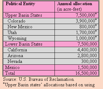
Arizona was especially disturbed about California’s growing water demands and did not ratify the compact until 1944, 22 years after it was initially negotiated. Arizona’s ratification of the compact was linked to the development of the Central Arizona Project, a 336-mile long system of aqueducts designed to deliver 1.8 MAF of water per year to the state’s southern growth area. However, before this project commenced, California and Arizona had to resolve their differences as to how much water each state would receive from the river. These differences resulted in an 11-year, complicated court case that eventually went to the U.S. Supreme Court. Finally, the case was resolved with California receiving 4.4 MAF, Arizona 2.8 MAF and Nevada .3 MAF. See Table 1. In addition, each state was allowed to use all the water in the tributaries located within the state’s boundaries. Relative to its population size, Arizona was the big winner in this case. In the early 1950s when the case was being litigated, Nevada did not visualize the recent rapid growth of Las Vegas and environs. Today, Nevada might argue for a larger allocation.
The Upper Basin states worked together in a more cooperative manner than the Lower Basin states and quickly formulated a contract that allotted 51.75% of the Upper Basin water to Colorado, 23% to Utah, 14% to Wyoming, and 11.25% to New Mexico. Percentages were used rather than actual amounts since the states did not know how much water would be available to the Upper Basin each year due to the combination of precipitation variability and the requirement of providing 9.0 MAF to the Lower Basin and Mexico.
TABLE 1: Colorado River Allocations
Precipitation Patterns
The arid and semiarid American Southwest constantly faces precipitation variability. What moisture the region receives to feed the Colorado River and its major tributaries, the Green River and San Juan River, is the result of various climatic conditions. A change in any one of these conditions could bring on a flood or drought. The Upper Basin falls mainly on the Colorado Plateau, which experiences both a winter and summer precipitation regime. In the basin’s higher elevations that form its headwaters precipitation falls rather evenly throughout the year, building large snowpacks during the cold months. Cold frontal systems developing over the North Pacific Ocean bring large amounts of precipitation during the winter and spring months. These systems acting like large rivers flowing eastward across western United States carry moisture at high levels in the atmosphere. As these atmospheric rivers encounter the high elevations of the Colorado Plateau, orographic conditions occur, resulting in increasing amounts of precipitation with the increase in elevation. In the San Juan, Uinta, and Wind River mountains these systems create large snowpacks that normally meltdown at a gradual rate during the late spring and early summer to provide water for the Colorado River throughout the summer and into the fall. If these winter frontal systems originate over warmer waters in the Pacific Ocean, precipitation in the form of rain might fall on the mountain snowpacks producing fast, high runoff and floods on the rivers.
During the summer regime rain over the Colorado River Basin comes from convectional systems. Low-level moisture arriving from the Gulf of Mexico, the Gulf of California, and the eastern Pacific Ocean generate thunderstorms in July and August. This atmospheric condition is referred to as the “North American monsoon,” and normally generates 30 to 40 percent of the annual rainfall in the Lower Basin where the rainfall ranges between 3 and 10 inches (76.2 and 254 mm) per year. These storms generally produce high-intensity rainfall in the Lower Basin where high summer temperatures and low elevations exist. Lower-intensity rainfall occurs more in the cooler and higher Upper Basin. These thunderstorms tend to be local in geographic coverage. They can create flash flooding but contribute little to the large rivers within the basin.
The factors producing the drought conditions throughout major areas of western United States including the Colorado River Basin are not fully understood. The expansion of the warm El Nińo ocean current within the equatorial portion of the Pacific Ocean has been associated with floods and droughts in western United States. Warm winter storms originating from warm ocean surfaces result in rapid meltdown of mountain snowpacks. Such meltdowns produce early above-average runoff followed by later below-average inflow into the basin. However, an El Nińo event normally lasts 6 to 18 months, not long enough to create the current six-year drought. Another factor might be an ocean temperature pattern occurring in the North Pacific Ocean outside the equatorial region. Called the Pacific Decadal Oscillation (PDO) it varies between a warm and cold cycle over a 30 to 50 year period. The causes behind the variations in the PDO are not known but recent research points out an association between the PDO phases with the above- and below-average precipitation and streamflow in the Colorado River Basin.
Annual Water Flow
Based on the 1922 Colorado River Compact, Lee’s Ferry, which is located just below the Glen Canyon Dam, separates the Upper Basin from the Lower Basin. Water flow data are collected at this point to measure the amount of water moving from the Upper Basin to the Lower Basin. Flow data has been measured or estimated at this point since 1885 but different measurement techniques have been employed over this long time period. From 1885 to 1922, estimated annual flow amounts were determined for Lee’s Ferry by E.C. LaRue, a U.S. Geological Survey engineer assigned to the Division of Water Utilization in the Southwest. From 1923 through 1962 stream gauges were used to determine the volume. In 1963 Glen Canyon Dam was completed; thus, from 1963 to present the measurements at Lee’s Ferry are assumed to approximate the total flow volume into Lake Powell.
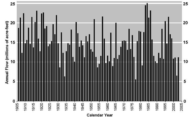
FIGURE 3: Estimates of Colorado River flow from 1906-2003. Source: U.S. Bureau of Reclamation.
Figure 3 illustrates this data set from 1906 to 2003. Measurements from 1905 to 1922 were used to ascertain the 15.0 MAF of water per year for the Colorado River Compact. The actual annual average during this period was 16.1 MAF, which was the highest long-term annual flow volume in the 20th century. During this period less annual variation in flow was recorded than for the period after 1922. The average annual flow during the seventeen-year period from 1986 to 2003 was 12.4 MAF, only 77 percent of the 16.1 MAF level from the seventeen-year period of 1905 to 1922.
Table 2: Average Flows During Recent Droughts
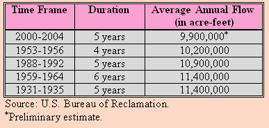
Since Lake Powell reached full capacity in 1980 the highest annual volume flow occurred in 1984 with 25 MAF and the lowest in 2002 with 6.8 MAF. Flow in the basin varies significantly from one year to another based mainly on precipitation amounts and a growing upstream water use. Within this variation certain drought periods can be identified. Table 2 shows the drought periods over the most recent 70-year time span. The 2000-2004 (now extending to 2006) drought has the lowest average annual flow. The 9.9 MAF figure is an estimated average. Between 2001 and 2003 the flow reached a low of 5.4 MAF. The duration of these droughts has been between 4 and 6 years, which might indicate an ending to the present drought. However, due to the low 2006 February precipitation levels within the basin, the U.S. National Weather Service predicts the April through July inflow to be 7.2 MAF, well below the average 9.9 MAF level for the drought. This low inflow is occurring at the time of the year when the greatest snowpack meltdown is taking place. Thus, the present drought does not appear to be ending. Also, between 1886 and 1904, an eighteen-year drought occurred, and tree-ring records over several centuries have revealed severe droughts lasting for decades.
Lake Powell’s Shrinkage
Figure 4 provides four Landsat 7 true color composite images of the lower portion of Lake Powell. The first image (top, left) was taken on October 10, 1999 when the reservoir contained 22,876,730 acre-feet of water. The current drought basically started at the time when this image was recorded. The other three images were taken near the beginning of June in the years 2000, 2002, and 2004. By June much of the spring runoff from the snowpacks in the surrounding mountains has made it to the lower portion of Lake Powell. After June the summer and fall inflow to the reservoir generally decreases. The summer monsoons are sporadic in their location across the basin and might provide some summer flashflood conditions but do not contribute significantly to the reservoir.
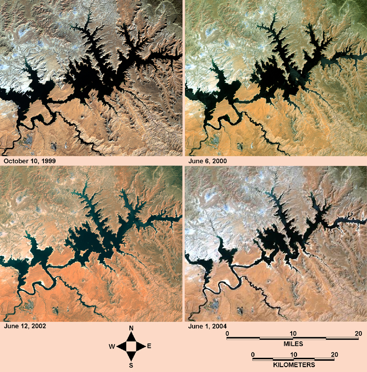
FIGURE 4: Landsat 7 images of Lake Powell at various times throughout the drought.
The four images illustrate the shrinking size of the reservoir between 1999 and 2004. In 1999, Wahweap Bay was at its full extent and Castle Rock Island occupied the center of the bay. Figure 5 shows the location of these geographic places. Not much change occurred in the bay between 1999 and 2000. On June 6, 2000 Lake Powell’s water level had dropped only to 21,385,072 acre-feet, approximately 1.5 MAF below the October 10, 1999 level. (These figures represent the recorded amounts for the entire reservoir on the indicated dates.) By June 12, 2002 the drought had lowered the reservoir to 16,427,414 acre-feet and Castle Rock Island was no longer an island. A land bridge appeared linking the island to the lake edge. Also in 2002, only a narrow inlet connected the upper and lower portions of Wahwaep Bay. By June 1, 2004, the reservoir was at 10,575,179 acre-feet, a 46.2 percent drop from the October 10, 1999 level. A wide land bridge closed the inlet and the two portions of the bay were now separated. Boats maintained in a marina located in the lower section of the bay now must enter the main channel of the Colorado River to reach the upper half of the bay. Antelope Island has merged with the mainland. Warm Creek Bay, just off of Wahweap Bay, shrank considerably within the four-year period.
In 1999 some small islands are located in Padre Bay, which is situated just upriver from Wahweap Bay. By June 2000, only nine months after the October 1999 image, these islands are noticeably larger in area. In the 2002 image some of these islands have coalesced and new islands have appeared as the reservoir’s water level continues to drop. By 2004, a large land bridge extends from Gunsight Butte to these islands, making for a continuous land body. By 2002 and especially by 2004, a white line outlines much of the edge of the reservoir. This line identifies exposed land that only a few years before was under water. A rather large section of this newly exposed land appears on the Colorado River directly across from Antelope Point. The water level had to drop 30 feet (9.1 m) to show this area.
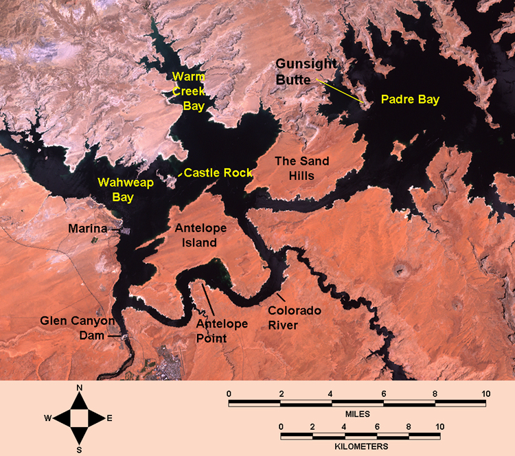
FIGURE 5: Selected geographic locations in the lower portion of Lake Powell.
The last time that Lake Powell’s water level was at this level occurred in May 1969 when the reservoir was still filling after the construction of Glen Canyon Dam in 1963. Seventeen years of normal inflow were required for the reservoir to reach its storage capacity. For the reservoir to return to this level again, eleven years of normal inflow would be needed. This time span does not take into consideration bringing Lake Mead back up to its capacity, which is presently at 54 percent, and the continuing growth and development within the basin. Some speculation exists that both Lake Mead and Lake Powell will never refill to their capacity levels.
In addition to not being able to provide freshwater to farms and cities, Lake Powell might have to stop production of hydroelectricity. Glen Canyon Power, which operates the dam’s power facilities, has indicated that if the present drought continues, it will not be able to generate electricity by 2007. At full capacity, Lake Powell produces enough electricity to power 1.5 million homes, mainly in Arizona and New Mexico.
The Lower Basin states and Mexico continue to receive their combined 9.0 MAF of water per year. The Upper Basin states are now challenging the requirement of providing 7.5 MAF to the Lower Basin states each year, pointing out that according to the compact they must deliver 75 MAF every decade and they have provided in some decades surplus amounts of water. They also argue that the Lower Basin tributaries should be used to provide some of the water for Mexico. The Upper Basin possesses some leverage in trying to make adjustments in the compact. If Lake Powell cannot produce electricity, it is mainly the Lower Basin that will suffer.
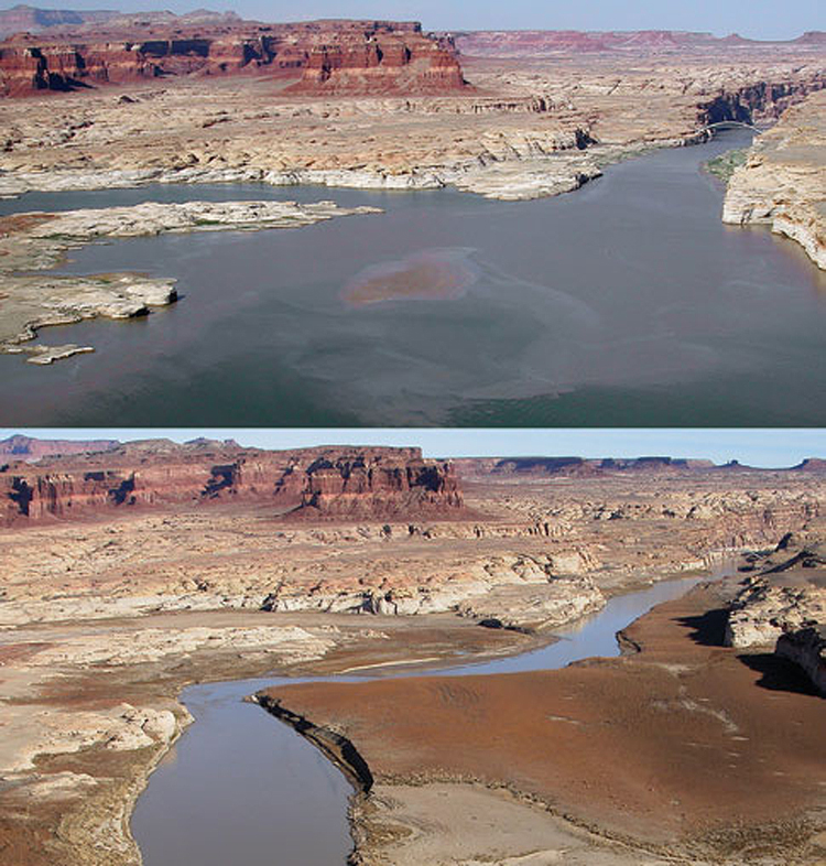
FIGURE 6: Eighteen month change in Lake Powell. (Photographs by John C. Dohrenwend, Courtesy of the USGS)
Ground level photographs (Figure 6) demonstrate how severe the drought has become. The top photograph was taken on June 29, 2002; whereas, the bottom photograph was recorded 18 months later on December 23, 2003.
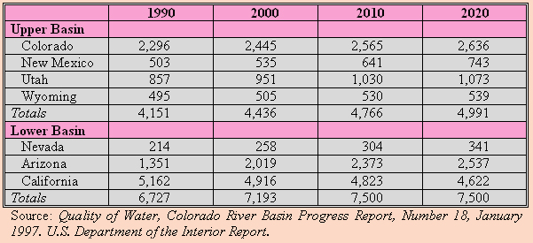
Future Growth
Table 3 shows the actual water used in 1990 and 2000 by each state within the basin and the projected usages for 2010 and 2020. The Lower Basin has almost reached its full water allocation of 7.5 MAF per year. California is gradually lowering it usage but even by 2020 it still exceeds its allocation. Nevada will start exceeding its allocation by 2010. Only Arizona remains below its allocation but its usage is increasing. Agriculture consumes about 80 percent of the state’s allocation. California and Nevada are presently using Arizona’s surplus water. The question has been raised, “Why should the Upper Basin, more specifically Lake Powell, release water that allows California and Nevada to exceed their allocations?” The Upper Basin states remain well below their allocations but their water needs are gradually increasing. In 2000 the basin states used 11.6 MAF of water; this number increases to 12.2 MAF by 2010. Although these amounts are still below 15 MAF of water established by the compact for the basin states, they are very close to the average annual inflow of 12.4 MAF recorded between 1986 and 2003, a time period that appears to more accurately reflect Lake Powell’s normal operational water level. Maybe with the severity of this drought and the dangerously low water level in Lake Powell, the time is appropriate for reconsidering the 15 MAF inflow figure.
TABLE 3: Colorado River Basin Depletion Projections (Unit: 1,000 acre-feet/year)
ANALYSIS:
Data Sets
This module uses two Landsat data sets, one recorded on October 10, 1999 and the other on June 13, 2002. The first data set was taken in the fourth quarter of 1999 when precipitation throughout the Upper Basin first started to decrease dramatically. Thus, this data set corresponds to the beginning of the drought. Lake Powell at this time was still 95 percent full. Taken about four years later the second data set clearly shows the impact of the drought on Lake Powell. This data set relates to the second quarter of the year when runoff from the mountain snowpacks should put the reservoir at the highest level for the year.
The two data sets cover the lower portion of the reservoir. It was possible to have the data sets dealing with the entire reservoir but they were too large for this instructional module. Each data set has 1320 scan lines and 1635 picture elements per image. The data sets were recorded by Landsat 7 using its ETM+ (Enhanced Thematic Mapper Plus) sensor. The data sets consist of the Landsat multispectral bands 1-5, 7. The pixel size for both data sets is 28.5m x 28.5m. Although the data sets are the same size, they are not geometrically rectified to each other; thus, they cannot be integrated. The second data set also has a DEM (Digital Elevation Model) layer that is geometrically rectified to the bands in the set. The DEM data were collected independently of the Landsat data.
The software programs, EarthScenes and Microsoft Paint, are used throughout this instructional module and all the functions required to complete the tasks associated with this exercise are available with these programs. EarthScenes is an image processing software program that provides various functions to enhance images, makes color composites, and classifies images. To use EarthScenes one must first create a master file that can hold twenty-five theme layers of information. A single band forms one theme layer. Paint is a graphics program that has a variety of tools to create, manipulate, and enhance graphic products.
Procedures
The objective of this exercise is to measure the impact of the drought on Lake Powell between 1999 and 2002. More specifically, the objective is to determine the surface area of the lower portion of the reservoir when the drought started and the amount of change in the surface condition of the reservoir four years into the drought.
First, create a master data file in EarthScenes for each data set and load the six multispectral bands into the respective files. Also, enter the DEM data into the 2002 master file. As previously indicated the size of a data layer in the master files is 1320 scan lines by 1635 pixel elements. To create a master data file, click “File” on the main menu bar followed by “Create the data files for a new image.” The program will want to know the directory path and the name being given to the master file and some bookkeeping files. Once the master file is created, load the individual band files by clicking “File” again followed by “Import layer data for a new image.” Use the “Import BMP images” option to load the individual band files.
1999 Data Set
Next, using the 1999 master file, create a histogram for each of the bands. Since this exercise is based primarily on bands 1-4, the next step is to contrast stretch these bands to expand their data ranges over the full possible data range, which is 1 to 250. Save the stretched bands as new layers in the master file. One can contrast stretch a band by using its existing minimum and maximum data values but a better enhancement of the band might be accomplished by analyzing the distribution of the data and using different minimum and maximum values. For example, the minimum and maximum values for Band 3 of the 1999 data set are 17 to 231. By plotting the histogram one can see that most of the data values are concentrated and very few values exist at the upper level of the histogram. By using the arrow keys on the keyboard one can find out the data value of each bar on the histogram. In this example, the new minimum and maximum values selected were 18 and 218. This range accounts for 99.9% of the entire actual data range and will create a greater gray-tone contrast of the image than the original minimum and maximum values.
Once bands 1-4 have been enhanced by stretching the data range, produce a true color composite by using the stretched bands 3, 2, and 1 to correspond to the colors red, green, and blue. Color composites are saved in a second master file designed to handle such images. Now export this true color image in color composite BMP format. EarthScenes will ask for the three bands to be identified again and will then produce a 24-bit BMP file and store it in the selected directory under the name provided. Figure 7 shows the 1999 true color composite for the lower portion of Lake Powell. Minimize EarthScenes and start Paint. Load 24-bit BMP file into Paint and minimize this program.
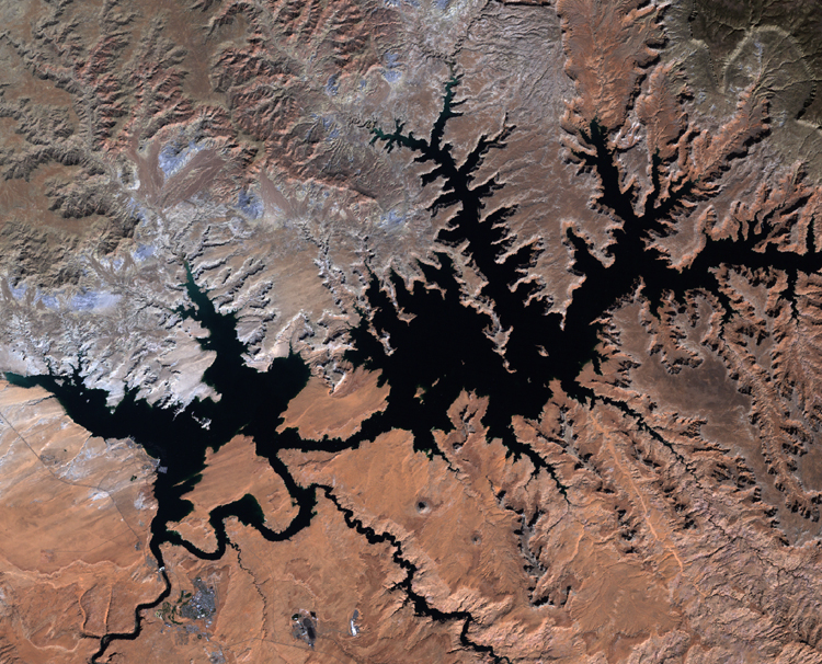
FIGURE 7: 1999 True color composite.
Maximize EarthScenes and contrast stretch Band 4 in the same manner used for bands 1 to 3. In this particular case a minimum of 12 and maximum of 180 were used. Create a histogram of this stretched band and plot the histogram. Note that the histogram has two concentrations. The very narrow, tall concentration at the lower end of the diagram relates mainly to the water conditions on the image. As a near infrared band, Band 4 does an excellent job of separating water from land. It does not show much variation within the water. A dip in the histogram occurs between the two concentrations, which represents transitional conditions between water and land. Some of this transitional area might correspond to wet surfaces around the edge of the reservoir. The second concentration, that is lower but broader than the first one, relates to land conditions and the variation within land surfaces.
The next step is to produce a two-class density slice classification of the stretched Band 4. The first class will be for water and the second class for all other surfaces. From the main menu, click on “Classify” and then “Density slice.” Select “Window and layer processing.” The input layer is the contrast stretched Band 4 layer. On the next menu select the “Default classification colors” and then select an output layer. Use one of unoccupied layers for the output layer and give it a name. This is where the classified file will be placed. The histogram now appears for the input band with a set of instructions. Press the Ins key on the keyboard to start the classification. Using the right arrow key, move over to the data value 13. The bars between 1 and 13 will be made red. This is the water class. Press the Ins key to stop the classification for the first class. Press the Ins key again to start the classification for the second class. Since there are only two classes, move the right arrow key all the way to the end of the histogram. The bars will be made green. At the end of the histogram, press the Del key to terminate the classification process. Several menus will appear that can be ignored. The classified image will be in red and green. It can be fully viewed by using the “Single layer pan and roam” option under “Display.”
To make the classified image usable for the next operation the colors on the image need to be changed. Click on the “Look-up-tables” followed by “Create a p or c color table.” Click on “Classification” and provide a name for the color table file. A window entitled “Get Classification Colors” will appear with Class 1 highlighted. Click the “OK” button which will provide a color palate. Select the bight blue color for water and click “OK” again. Repeat this process for Class 2 but select white for the color. After completing the second color, click on the “Finish selecting colors” bar. Now click on the “Look-up-tables” followed this time by “Load a p or c color table.” Select one of the three “User Tables” buttons and then the name of the color file previously created.
Under “Display” choose the “Single layer through a look-up-table” option. Select the classified layer and then click on the appropriate “User Table” button. The classified layer will now have blue and white colors. Export this layer using the “Single layer BMP format.” Place this exported file in the same directory that contains the previously developed true color composite.
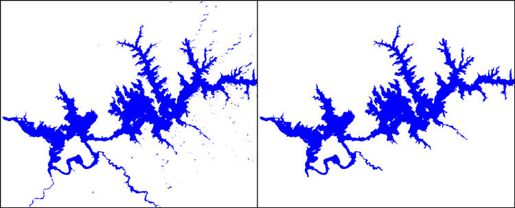
FIGURE 8:Classified Lake Powell (Left), Modified Classification (Right).
Minimize EarthScenes and start a second version of Paint. Load the classified file into this version of Paint. In looking at the classified file, one will note that patches of blue exist beyond the reservoir. These areas are mainly shadows from steep cliffs. These areas as well as the Colorado River below Glen Canyon Dam have to be removed since they do not relate to the water surface of Lake Powell. Click on red on the color palate. Using the Paint Bucket tool, click on the blue area within the reservoir. This blue area should become gray. Click on blue on the color palate. Again, using the Paint Bucket tool, make all the white areas, except those within the reservoir, blue in color. Change the color to white and make all of the blue areas white again. Now change the color to blue and click on the gray area. This procedure has now removed all of the non-reservoir blue areas. Figure 8 shows the before and after images of the classified file. Save the changed image.
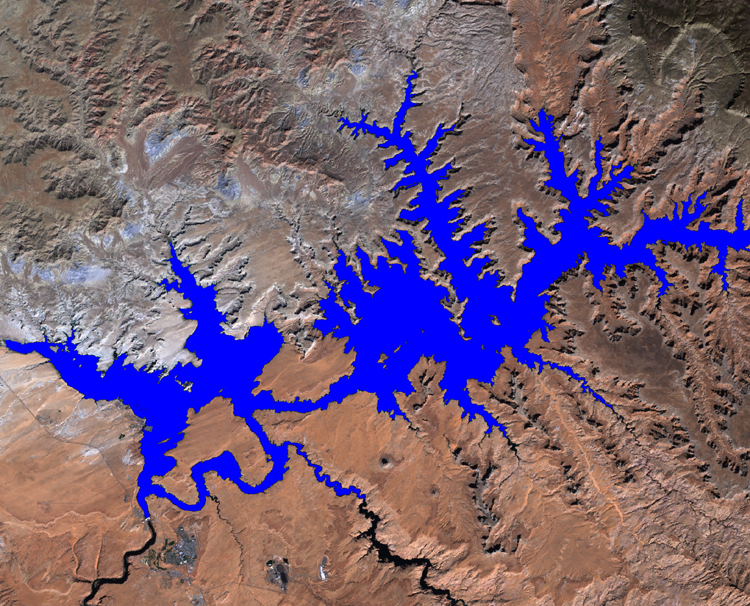
FIGURE 9: 1999 True color composite with Lake Powell superimposed
At this point two versions of Paint should be running. The first version contains the true color composite (Figure 7). The second version has the modified classification file showing Lake Powell in blue with white background. Move the vertical and horizontal bars to their uppermost and leftmost positions, respectively, on both versions of Paint. Do a “Select All” and “Copy.” of the classification file situated in the second version of Paint. Next, move to the version of Paint with the true color composite and do a “Paste.” Next, click on the transparent background button (last button in the tool box menu). The blue reservoir should now be superimposed on the true color composite with the remainder of the image showing the true color composite (Figure 9). Save this image under a new name as a 24-bit BMP file.
Now shut down the two versions of Paint and maximize EarthScenes. Using EarthScenes, input the 24-bit BMP file that was just saved. Click “File” on the main menu bar followed by “Import layer data for a new image.” Use the “Import BMP images” option to load the new file. This is the same procedure followed when loading the original data files. However, this time the program will breakup the 24-bit BMP file into three 8-bit BMP files associated with the red, green, and blue color layers of the 24-bit BMP file. Each of these layers will occupy a separate input layer on the master file.
Take time to view each of the new layers. Note that on the blue layer the reservoir is a bright white; whereas, other water areas are still dark. This separation does not exist on the red and green layers. Create a histogram of the blue layer and then plot the histogram. The plot shows the reservoir with the large number of data values related to the 250-bar on the histogram. Using this information, make a density slice classification of the blue layer. The classification will have two classes: 1-249 (non-reservoir) and 250 (reservoir). Once the classification is completed a window titled “Classification Areas” will appear. Copy the numbers recorded with each class. These numbers represent the number of pixels associated with each class. The non-reservoir class had 1,874,936 pixels and the reservoir class had 283,264. Recall that a pixel covers a 28.5m x 28.5m surface area. With this information, the amount of surface area within the lower portion of Lake Powell for October 10, 1999 can be calculated. The surface area is 88.83 square miles (142.9 sq. km.).
2002 Data Set
Repeat the steps used with the 1999 data set using the following parameters. Contrast stretch Band 4 by entering a minimum value of 8 and a maximum value of 168. Classify the contrast stretched Band 4 by using the density slice 1-32 for the water surface class and 33-250 for the non-water surface class. The 2002 image should correspond to Figure 10, which is the 2002 true color composite with the water surface transposed on it. Visually compare the 2002 image with the 1999 image to determine what portions of the reservoir have shrunk in area.
The MSS 1975 image creates some challenges with respect to finding reference points. First, as previously indicated, the image is fuzzy due to its original resolution (57 m x 57 m) being adjusted to the resolution of the other images (28.5 m x 28.5 m). Second, the image contains line striping, a typical problem associated with Landsat MSS data. The striping will appear mainly over the white ice field area. Third, a diagonal line cuts across the image. It is an individual scan line problem and does not represent a problem for locating reference points. Finally, the image might appear dark. To overcome partially this problem one can enhance the bands by stretching the data. This is accomplished by using the “Contrast stretch” function. However, before using this function histograms have to be created for the appropriate bands. Use the “Create the histogram” function to complete this task.
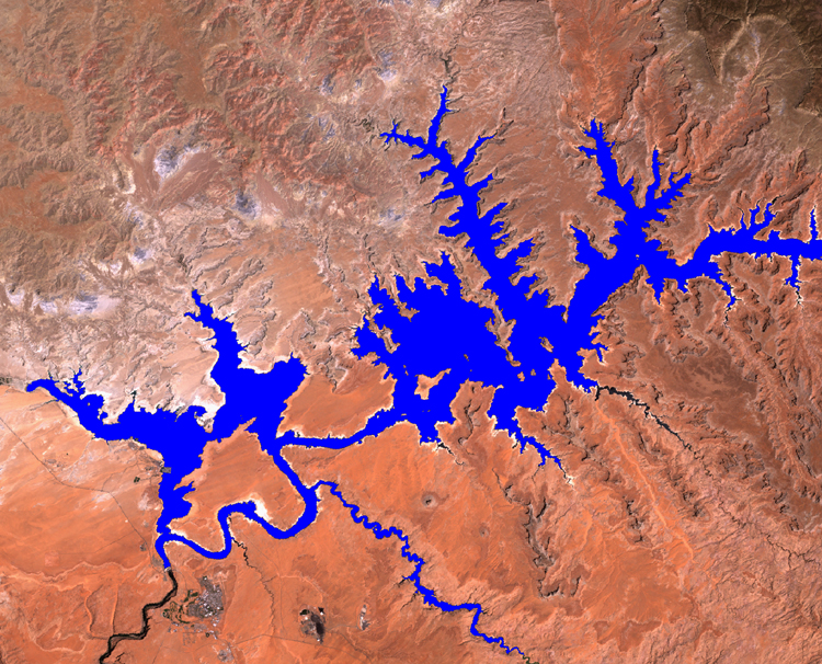
FIGURE 10: 2002 True color composite with Lake Powell superimposed
Repeat the steps used with the 1999 data set using the following parameters. Contrast stretch Band 4 by entering a minimum value of 8 and a maximum value of 168. Classify the contrast stretched Band 4 by using the density slice 1-32 for the water surface class and 33-250 for the non-water surface class. The 2002 image should correspond to Figure 10, which is the 2002 true color composite with the water surface transposed on it. Visually compare the 2002 image with the 1999 image to determine what portions of the reservoir have shrunk in area. As with the 1999 image this image can be imported into EarthScenes and reclassified. The new classification will calculate the number of pixels associated with Lake Powell. With this information and knowing that a pixel is 28.5m x 28.5m in size, the water surface can be determined in terms of the number of acres and square miles.
Elevation data are available as part of the 2002 data set. Look at the histogram for the elevation layer and note that the pattern for the histogram is rather level except for one large spike that is associated with values 103 and 104. These values relate to the water elevation level of Lake Powell. Create a new color table file that will have three classes and assign the colors white, red, and white to the three classes. Load the new color file. Do a three class density slice classification of the elevation level using the ranges 1-102, 103-104, and 105-250. Display the new classified file using the new color table.
Employing the same procedures used in producing the 1999 and 2002 water surface layers, export the classified elevation file based on its new color table; use Paint to remove extraneous pixels (pixels at the same elevation as the reservoir but not associated with the reservoir area) from the classification file; and superimpose the modified elevation file on the 2002 true color composite. Import the modified classification file into EarthScenes as a new layer; make a histogram of the file; and reclassify it in order to obtain the number of pixels associated with the elevation of Lake Powell. The number should be 318,639 and with this number calculate the number of acres and square miles covered by the reservoir based on its normal elevation level. These numbers can be compared with the 1999 and 2002 water surface layers to ascertain how much the reservoir has decreased in size from its normal elevation level. Finally, overlay the 2002 water surface layer on the true color composite file that has the normal elevation level already superimposed on it. The final product should look like Figure 11.
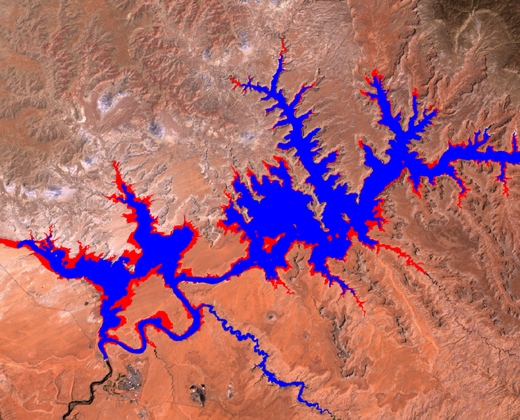
FIGURE 11: Normal elevation level for Lake Powell in red with 2002 water surface level superimposed.
Suggested Books:
Carothers, Steven W and Brian T. Brown, 1991, The Colorado River Through Grand Canyon, Tuscon: The University of Arizona Press.
Gelt, Joe, “Sharing Colorado River Water: History, Public Policy and the Colorado River Compact.” Arroyo, Vol. 10, No. 1, August 1997.
Topping, Gary, 1997,Glen Canyon and the San Juan Country, Moscow, Idaho: University of Idaho Press.
Webb, Robert H., 1996,Grand Canyon: A Century of Change, Tucson: The University of Arizona Press.