
MAP MAKING IN THE INFORMATION AGE
Prof. Paul R. Baumann
Department of Geography
State University of New York
College at Oneonta
Oneonta, NY 13820
COPYRIGHT © 2001 Paul R. Baumann
INTRODUCTION:
As the World rapidly enters the Information Age, the need for better and up-to-date maps becomes essential. People are finding it difficult, through the traditional written methods of communication, to absorb all the items with which they must deal during this new age. Basically, they are being overwhelmed with information. To handle partially this situation, more and more information is being presented graphically rather than textually. The map is a graphical communication medium by which a tremendous amount of information can be conveyed quickly. However, in order for the map to be an effective means of communication, it must be understood and it must be up-to-date and accurate.
For more than two decades British educator William Balchin has promoted the idea that K-12 school curricula should include geography with English and mathematics as foundation subjects. He notes that the four types of basic intelligence - verbal, social, numerical, and visual-spatial - relate to literacy, articulacy, numeracy, and graphicacy. He defines graphicacy as “the communication of spatial information that cannot be conveyed adequately by verbal or numerical means.” The tools of graphicacy are maps, diagrams, photographs, and other spatial documents.
Many maps are not accurate and are out-of-date, which can create problems for people using them to make decisions. It is a very difficult and time-consuming task to keep maps accurate and current. Like other map agencies throughout the world, the United States Geological Survey (USGS) is constantly striving to address this problem. In one map series alone it has to deal with the more than 54,000 large-scale topographic maps covering the 48 contiguous States and Hawaii. Remotely sensed imagery has become a valuable means for keeping maps accurate and up-to-date.
The goal of this instructional module is to present a methodology for updating the location and size of certain water bodies within a particular area of a USGS 7.5 minute topographic map. This methodology employs a Landsat TM (Thematic Mapper) data set, which covers a study area of 96.3 square miles or 249.5 square kilometers. The data set depicts conditions present on May 29, 1994 over the Kossuth, Indiana USGS topographic sheet. The USGS 7.5 Minute Topographic Quadrangle(Map)for Kossuth was originally produced in 1963, photorevised in 1980, and updated with minor revision in 1994.
BACKGROUND:
KOSSUTH TOPOGRAPHIC MAP
The Kossuth USGS 7.5-minute topographic sheet is situated in the northern portion of Washington County, in southern Indiana. The Kossuth topographic sheet is typical of most of the USGS maps throughout the United States in that it covers a landscape which is not particularly spectacular but nonetheless interesting. The area is very rural with the major community being the hamlet of Kossuth (population 50, 1990). Some of the more appealing place names found on the map sheet, which reflect the southern Indiana milieu, are Potato Knob, Crossroads Church, Pumpkin Center, and Suicide Cave. Figure 1 is a generalized map (scale 1:250,000), which covers the Kossuth topographic sheet and beyond. Click on this map and the Kossuth 7.5-minute topographic sheet will appear. This is a large file, which may take a few monuments to display.
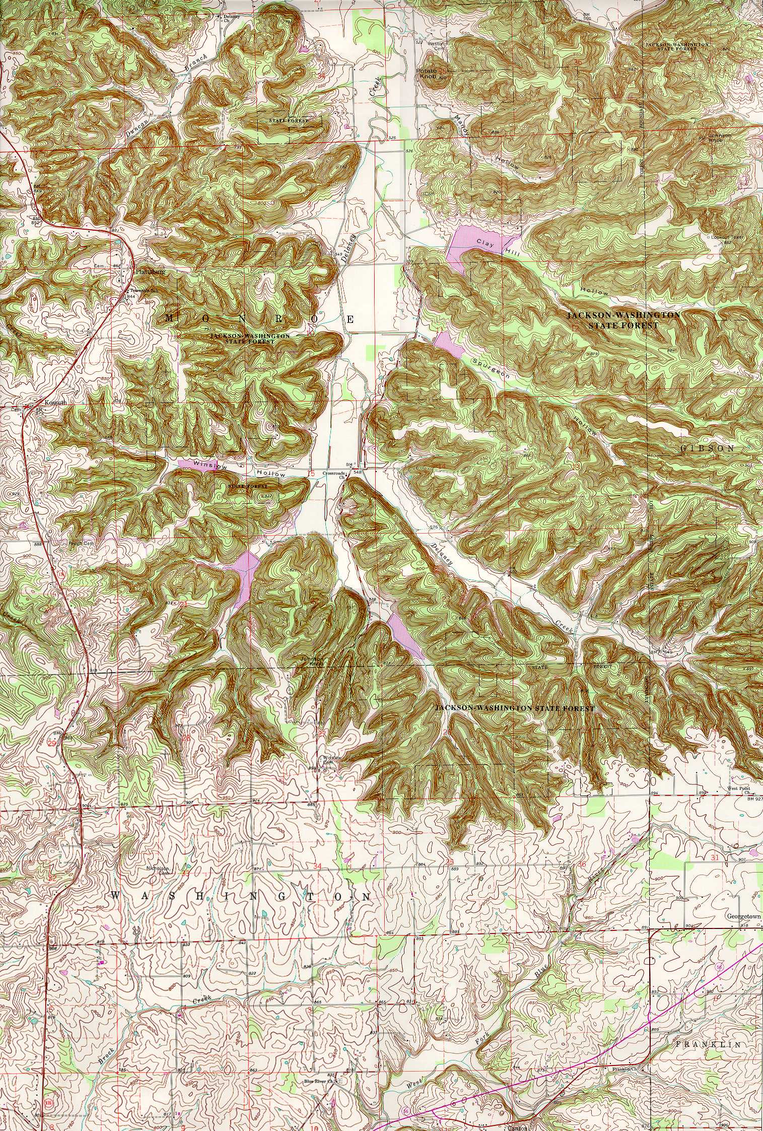
FIGURE 1
The most prominent landscape feature on the Kossuth USGS 7.5 minute topographic map is the Delaney Creek valley with the surrounding roughly dissected uplands. The valley floor is relatively flat and ranges from 550 to 600 feet in elevation. Deciduous trees grow along Delaney Creek, and corn and soybean fields cover the lower portions of the valley. Small fields of tobacco exist near the edges of the valley. The creek with its many small tributaries forms a classical dendritic drainage pattern. The uplands sharply rise from the valley floor and reach elevations of 850 to 900 feet. Mainly mixed forests of deciduous and evergreen trees cover them. Most of the area falls within the Jackson-Washington State Forest.
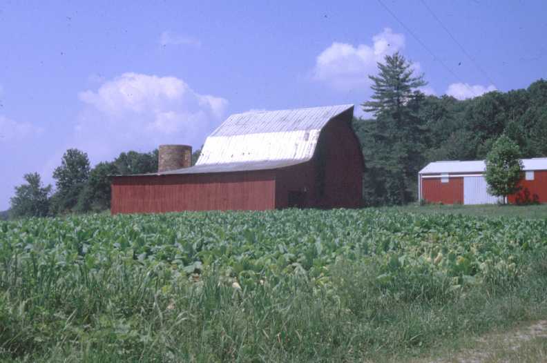
FIGURE 2
Figure 2 shows the typical small tobacco field with the uplands immediately behind it. This section of Indiana rests at the northern edge of the Kentucky tobacco region. Many old families in this section of Indiana trace their heritage back to Virginia by way of Kentucky. In such families tobacco has been a cash crop for generations and it has become as much a habit to grow it as to smoke and chew it.
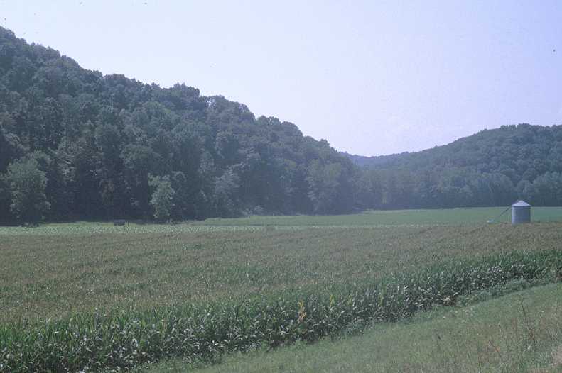
FIGURE 3
In Figure 3 a cornfield spreads across the valley bottom. Note the sudden contrast in slope and elevation between the valley bottom and the uplands. Also, note the haze over the hills, which generally indicates the beginning of a late summer, afternoon thunderstorm. This type of haze makes it difficult to obtain sharp satellite imagery over this region in the late summer. In addition, the heavy cover of green crops reduces significantly the contrast between the valley floor and the uplands. The imagery used in the module was taken in late May when the crops in the fields have just started to appear and most of the land cover is still bare ground, which helps to differentiate the valley floor from the uplands. See Figure 6.
The Kossuth topographic map cuts across three physiographic regions. The Scottsburg Lowland extends along the northern edge of the map. This is a low (500 to 550 feet), flat area on which the Muscatatuck River meanders. Muscatatuck does not appear on the map but can be seen on the data set imagery. The Delaney Creek flows northward into the Muscatatuck, which eventually enters the East Fork of the White River and then the Wabash. The Norman Uplands occupy the major portion of the map area. Along the edge of the Norman Uplands and Scottsburg Lowland is the Knobstone escarpment, which has thin beds of soft fine-grained bluish-gray sandstones and shales. These sandstones and shales erode easily and are responsible for the deep dissections into the Norman Upland, which are clearly evident on the map. The southern portion of the map relates to the Mitchell Plain. This is a limestone plain, which dips quickly away from the Norman Uplands. As one drives south out of the Delaney Creek valley, one is crossing a divide where the Blue River starts its southern journey to the Ohio River. The Mitchell Plain with its limestone formations is a karst region with caves and sinkholes. Some of the small, dot size ponds on the bottom section of the topographic map are sinkholes with water in them. Figure 4 shows the major physiographic regions of southern Indiana with the political boundaries of Washington County superimposed on the three regions just described. It also identifies the location of the southern boundaries of the Illinoian and Wisconsin glaciers. The continental glaciers never covered a large section of southern Indiana, including most of Washington County.

FIGURE 4
The Kossuth topographic map shows several reservoirs nestled into the tributary valleys (hollows) entering the Delaney Creek valley. The reservoirs are colored purple on the map, which means that they were added to the map at a later date. The information on the reservoirs was obtained from aerial photographs and other sources but the information was not field checked. The reservoirs provide flood control for the Delaney Creek valley. With the steep slopes of the uplands and the frequent heavy summer thunderstorms associated with southern Indiana, small but devastating floods can occur suddenly in the valley area. The large reservoir (Figure 5) in Clay Hill Hollow is also used for recreation and forms the heart of Delaney Creek Park, which is maintained by the county. Note that the reservoirs are situated on the valley floor and are covering good farmland.
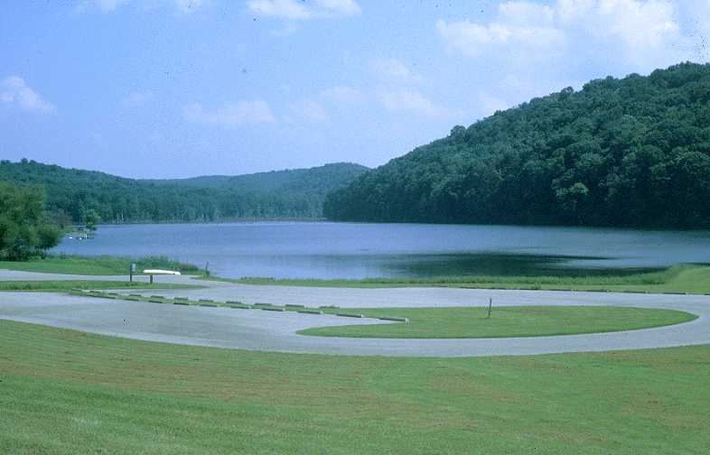
FIGURE 5
WATER BODIES
The Kossuth map was originally produced in 1963 and photorevised in 1980. As previously indicated,
producing an accurate and up-to-date map is a long and complex process. It normally takes five years from the
identification of a USGS 7.5 minute mapping project to the printing of the final map. This process requires a
team of professionals and a series of closely coordinated steps. It used to take longer to produce a map because
much of the needed information was gathered by field work and surveying, which are very expensive procedures. In
recent decades the USGS has turned more toward aerial photography to obtain the required information. Most photographs
used for the USGS’s topographic mapping program are now acquired through the National Aerial Photography Program (NAPP).
NAPP flights are flown in a north-south direction along carefully determined flight lines. It takes 10 precisely
positioned NAPP aerial photographs to provide the stereoscope coverage needed for each 7.5 minute map. At this
coverage level NAPP photographs are mainly at the scale of 1:40,000. They are also generally black-and-white
photographs. At this scale and with only black-and-white photographs an aerial photo interpreter might overlook
some features. An examination of the satellite data set (Figure 6) being used in this module shows the location of several
more reservoirs in the Delaney Creek valley, which do not appear on the 1980 photorevised map. These reservoirs
could have been built after 1980, and thus, would not appear on the NAPP photographs. However, the map states that
“minor revisions” were made in 1994, the year that the satellite data set was acquired. The minor revisions were
noted on the map in the following manner:
“Photoinspected from 1992 source; no major culture or The missing reservoirs probably were not constructed within the two year period between 1992, the date of the
photo source, and 1994, the date of the satellite imagery. It would take several years to build and fill
such reservoirs. It would also take time for vegetation to cover the earth dams and other disturbed lands around the reservoirs.
Disturbed land surfaces would produce bright reflectances on the imagery. No such reflectances occur around these reservoirs
indicating no recent construction. In addition, the minor revisions were dated 1994. Funds for building these reservoirs came from
the Soil Conservation Service of the U.S. Department of Agriculture; thus, their existence had
to be known. The problem most likely rests with the pressure and demand to provide up-to-date
information, in this case map information, without giving full consideration to accuracy.
drainage changes observed. Boundaries revised and names
verified 1994.”
FIGURE 6
The objective of this module is to locate and measure these missing reservoirs using satellite imagery.
Figure 6 is a false color composite image of the study area. The bright red areas indicate healthy, green vegetation, and
correspond mainly to the forested uplands. The gray areas are related to bare agricultural fields found basically in the
lowlands. The black areas are water bodies. Note that the dam areas immediately in front of the reservoirs are also
bright red. These are earth dams with grass vegetation growing on them. Concrete dams would have a quite different
reflectance. Two yellow boxes outline the reservoirs that do not appear on the topographic map. Check these
areas with the full topographic map provided by clicking on Figure 1.
DATA SETS
The main data set employed in this module was acquired on May 29, 1994 by Landsat-5 using its TM sensor. The TM sensor collects data based on a 30 x 30 meter ground resolution cell for each of its bands except the thermal band, which has a 120 x 120 meter resolution. A ground cell is referred to as a picture element (pixel) when dealing with imagery. The data set is 640 by 480 pixels in total size. Many TM data sets are geometrically registered to the Space Oblique Mercator (SOM) cartographic projection, which is the case with this particular data set. This rectification results in the pixel size being 28.5 x 28.5 meters rather than the original size of 30 x 30 meters. The TM sensor records in seven sections of the electromagnetic spectrum. These sections are called spectral bands and a band has a distinct wavelength. Table 1 lists the seven TM bands along with their wavelengths and locations. Radiometrically, TM converts its analog-to-digital signal over a range of 256 digital numbers, which relates to eight binary bits or one computer byte. In other words, each pixel in each band has a value between 0 and 255. These values are measurements of reflected or emitted energy.
This module has a second data set, which covers the same geographic area and was also acquired on May 29, 1994, by another satellite. The second satellite was the IRS-1B, which is maintained by the National Remote Sensing Agency of India. This satellite collects data with three Linear Self Scanning Sensors (LISS-I and LISS-II a and b) at 72 x 72 meter and 36.25 x 36.25 meter spatial resolution. A data set has four spectral bands, all of which are nearly identical to the TM visible and near-infrared bands. See Table 1. The particular data set for this lesson was acquired by the LISS-II b sensor. This data set, like the TM data set, was geometrically registered to the SOM projection making its pixel size 36 x 36 meters. However, radiometrically the data range between 0 and 127 and are not as sensitive to variations in reflected energy as the TM data. The results of the second data set will be compared to the findings from the TM data set. Due to its higher spatial resolution and wider spectral data range, the TM data set has better quality data.
| Band |
Wavelength | Spectral Location | Band |
Wavelength | Spectral Location |
| 1 | 0.45-0.52 µm | Blue Visible | 1 | 0.45-0.52 µm | Blue Visible |
| 2 | 0.52-0.60 µm | Green Visible | 2 | 0.52-0.59 µm | Green Visible |
| 3 | 0.63-0.69 µm | Red Visible | 3 | 0.62-0.68 µm | Red Visible |
| 4 | 0.76-0.90 µm | Near Infrared | 4 | 0.77-0.86 µm | Near Infrared |
| 5 | 1.55-1.75 µm | Mid-Infrared | |||
| 6 | 10.4-12.5 µm | Thermal Infrared | |||
| 7 | 2.08-2.35 µm | Mid-Infrared |
ANALYSIS:
The first thing to be done is to select an appropriate band to be used throughout the analysis. An examination of the seven Thematic Mapper (TM) bands shows that the three visible bands (1-3), even when stretched, provide little evidence of the various water surfaces across the image. Band 4, the near infrared band, clearly separates water bodies from other surfaces and this differentiation is more apparent when the band is stretched. Band 5, a mid-infrared band, also differentiates between water bodies and other surfaces but the separation is not as strong as Band 4. Due to its spatial resolution and limited spectral data range Band 6 is not an acceptable choice for this project. Band 7, another mid-infrared band, is too dark and does not differentiate water well from other surfaces. Thus, Band 4, by far, is the best band for undertaking this project. Figure 7 shows four bands within the data set. Starting in the upper left and moving clockwise, the bands are 1, 3, 4, and 5, respectively. Band 4 stands out from the bands especially in detecting water.
FIGURE 7
The next step is to stretch Band 4. The minimum and maximum values are 6 and 167 respectively and they are stretched to 1 and 250. An examination of the histogram of the stretched band clearly shows that most of the data values are clustered in the upper portion of the histogram from 90 and above. The lower portion of the histogram contains a small cluster in the very low end of the value range followed by a rather straight-line pattern. The small cluster represents the main portions of the water bodies and a portion of the straight-line pattern corresponds to the edge areas of the water and other wet surfaces.

Using the software’s pixel read-out and zoom function (Figure 8), the value range for water can be determined. The low values of 1 to 15 are obviously water but it becomes difficult to ascertain the upper value for the edge areas of the water bodies. After checking several of the water bodies an upper level value of 70 was selected. One might select a different upper level value producing slightly different results. Once this value is determined, the next step is to do a density slice classification of Band 4, the stretched version. This will be a two-level classification with the first class being water (data range 1-70) and the second class being non-water surfaces (date range 71-250). This classification is saved as a new layer file within the software’s data base. This new layer has data values of only “1s”(water) and “2s”(non-water). In addition to the classified image, the classification produced a count of the number of data (pixel) values associated with each class. These numbers were 2,410 and 304,790 for class 1 and 2, respectively.
FIGURE 8
Figure 9 shows the classified image from the density slice classification. The color blue represents the water bodies across the image and the color green relates to all other surfaces. This classification clearly detects all of the major water surfaces within the Delaney Creek valley, not only those shown on the topographic map but also those shown on the infrared image. In addition, some of the water bodies cover larger areas than indicated on the map.

FIGURE 9

The new classified layer is now exported as a bitmap (.BMP) file so that it can be viewed and modified in Microsoft Paint. Load the bitmap file into Paint and edit two of the colors on the color box. Select Custom Colors under Edit Color (Figure 10). Develop two gray-tone colors by inserting the same value in each of the three boxes for red, green, and blue. The minimum and maximum value levels are 0 and 255. Do not select 1 or 2 since they already relate to the existing classes. It is best to select something like 50 and 100. Once the two new gray colors have been developed and their values known, use Paint’s brush function to paint the reservoirs within the Delaney Creek valley. Use one of the gray-tone colors to paint all the reservoirs within the valley that appear on the Kossuth topographic map. Use the second gray-tone color to paint the new reservoirs within the valley that appear on the image but not the map. With the brush function this step should take less than a minute to complete. Save the modified bitmap file.
FIGURE 10
Return to the image processing software and import the bitmap modified file into the software’s data base as a new layer. Next, do a four-class density slice classification on the new layer. Assign the first color to the data value of 1, which now relates to all the water bodies shown on the image outside the Delaney Creek valley. Select the second color for the data value of 2, which corresponds to the non-water areas throughout the image. The last two colors are assigned to the gray-tone values used in Paint to separate the reservoirs. This density slice classification will produce a new classified image file, which will be saved in the software’s data base. This layer will have values ranging from 1 to 4, corresponding to the four classes. A pixel count is also generated, which in this case has 1,364 pixels for class 1 (water areas outside the valley), 304,790 pixels for class 2 (non-water bodies), 209 pixels for class 3 (the new reservoirs shown on the image), and 837 pixels for class 4 (the reservoirs shown on the topographic map). See Figure 11. These pixel values can be converted into standard area measurements (Table 2).
FIGURE 11
The area measurements in Table 2 were ascertained by first determining the number of square feet in one pixel. One meter equals 39.37 inches or 3.28 feet. The number of feet, 3.28, is multiplied by the number of meters along one side of a pixel, which is 28.5 for the TM data set. This calculation provides the number of feet along one side of a pixel, which is 93.48. This number is squared to obtain the total number of square feet in one pixel (8738.51), which is then divided by 43,560, the number of square feet in an acre, to determine the proportion of an acre covered by one pixel. This proportion (0.200608) is finally multiplied by the number of pixels in each land cover class to obtain the number of acres in each class. For example,
Multiply the number of acres by .4047 to obtain the number of hectares.
| Pixels |
Acres | Hectares | |
| Class 1 | 1,364 | 273.77 | 110.79 |
| Class 2 | 304,790 | 61,174.56 | 24,757.34 |
| Class 3 | 209 | 41.95 | 16.97 |
| Class 4 | 837 | 167.99 | 67.98 |
Although both data sets are the same size with respect to the number of elements and lines (640 x 480), the LISS-II data set covers a larger geographic area due to its larger pixel size. This point must be considered when examining the area measurements in Table 3. Class 1, reservoirs and other water bodies outside the Delaney Creek valley, has more area identified as water since it extends geographically beyond the area associated with the TM data set and incorporates additional water area. The same situation holds true for Class 2, non-water areas.
Classes 3 and 4 are centered on the reservoirs in the Delaney Creek valley, which is situated in the middle of both data sets. Thus, the geographic difference in coverage by the two data sets should play a minor role in the area measurements for these two classes. In fact, the area measurements from both satellites are identical for Class 3, the new reservoirs. However, a 6.54 acre (2.65 hectare) difference exists for Class 4, the older reservoirs. This difference might be due to several factors. One factor might relate to the size of a pixel. The numerical value associated with a pixel is an average of the ground cell's surface reflectance. If a large portion, but not all, of a pixel covers a water surface, and thereby, generates a data value identified with water, the area of the entire pixel is then classified as water. This situation might add to the number of pixels being grouped with the water class. It is less of a problem in dealing with smaller pixels. The second factor might be due to the size of the wetlands areas found at the end of some of the older reservoirs. Determining the cut-off point between wetland areas and water areas is very difficult in a density slice classification. A different cut-off point for water might produce better results. The new reservoirs do not appear to have any major wetlands. A final factor might be the time of day when the two satellites crossed the study area. The sun elevation at the time that Landsat 5 passed over was 59 degrees; whereas, the sun elevation for the IRS-1B satellite was 70 degrees. The difference in sun elevation might create a difference in reflectance conditions.
| Pixels |
Acres | Hectares | Pixels |
Acres | Hectares | |
| Class 1 | 1,364 | 273.77 | 110.79 | 1,751 | 560.75 | 226.93 |
| Class 2 | 304,790 | 61,174.56 | 24,757.34 | 304,733 | 97,602.72 | 39,499.82 |
| Class 3 | 209 | 41.95 | 16.97 | 131 | 41.95 | 16.97 |
| Class 4 | 837 | 167.99 | 67.98 | 545 | 174.53 | 70.63 |
Figure 12 illustrates graphically the results of the two classifications for the Delaney Creek valley area. The results are basically identical. The TM classified image is a larger scale than the LISS-II B because it covers a smaller geographic area, and thereby, provides more detail.
FIGURE 12
This lack of accurate and up-to-date information on the Kossuth topographic map as well as other maps could be avoided if the USGS would use satellite data on a regular basis in conjunction with aerial photography in updating maps. Water surfaces are basic map features and are, in general, easy to detect on near infrared satellite imagery. Several remote sensing satellites provide such imagery. In addition, satellite imagery gives a synoptic overview of a topographic map surface in comparison to trying to mosaic ten or more aerial photographs.
Water surfaces are basic map features on topographic maps, which should be conveyed in an
accurate and up-to-date manner.
MATERIALS AND REFERENCES:
Kossuth, Indiana, United States Geological Survey 7.5 Minute Topographic Quadrangle (Map) corresponds directly with the data sets in area and clearly helps in identifying various physical and cultural features.