METEOROLOGY 361 Spring, 2014

The Case of the Two Clippers – Analysis using IDV

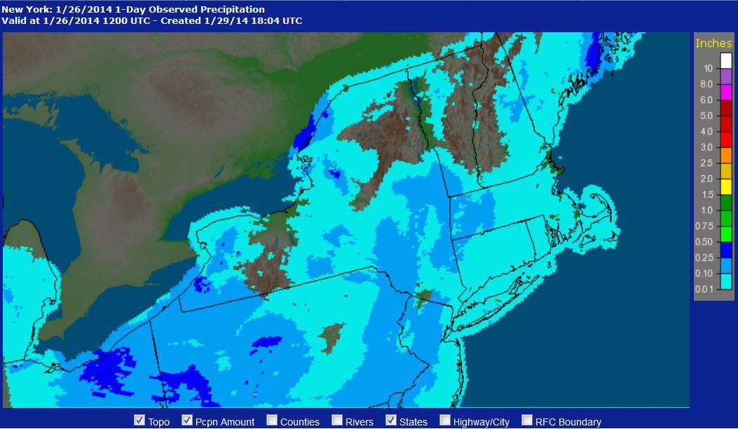
Last semester we were introduced to the Integrated Data Viewer (IDV), looking at a coastal storm that produced freezing precipitation. Next week we’ll use the IDV to look at a nor’easter with snow. For this lab we go back to the IDV to solve a meteorological mystery involving Clippers. On January 23, 2014 an Alberta Clipper formed in western Canada. This storm followed a Clipper track and exited the U.S. three days later, bringing a severe Arctic cold wave behind it. Also typical for these kinds of storms, there was very little snowfall. In Oneonta 1 inch of snow fell on January 25. On the same day, Boston received 0.1 inches of snow but only a trace of precipitation so it was almost nothing.

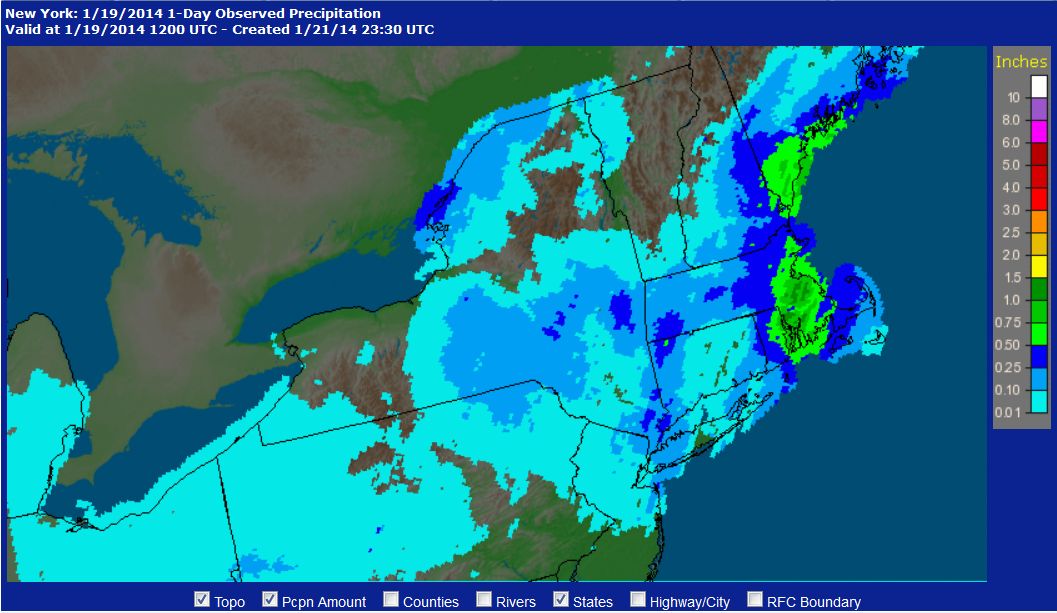
Just a week before, on January 15, 2014, a similar scenario had presented itself. That time, however, the Clipper produced a swath of snowfall that included 4 inches at Oneonta on January 18. Boston had 2 inches of snow but 0.79 inches of liquid so most of the precipitation was rain.

Both storms pursued essentially the same track southeastward to the Midwestern U.S. Both storms brought intense cold to the U.S. in their wakes. But the earlier storm was a snow producer, contrary to conventional wisdom about Alberta Clippers. What was different?

Procedure –

1. Go into the computer lab, room 308 and pick any computer other than the older ones in the front used for maps and observations only. Log on using your Oneonta username and password.

2. In the METR 360 folder (File System->Home->METR360) open the ClipperLab folder. There will be a Word file with these instructions. You also have AHPS maps of the liquid equivalent precipitation for both cases (AHPS precip analysis Jan 19 and AHPS precip analysis Jan 26). There are animated gif loops, one for each storm showing the surface maps (USsfcLoop Jan 18 and USsfcLoop Jan 25). You may click the links or run the loops with the OpenOffice equivalent of PowerPoint, called Impress.

3. Start the IDV from the applications menu. Be sure you have version 4.1, not the earlier versions. Go to the Dashboard and click Data Choosers, then click Files. If not already there, navigate to the ClipperLab folder again. Inside that folder are two zidv files for Jan 18 and Jan 25. You need to put the IDV Dashboard selector on one of the zidv files for these cases and click the Add Source button. It doesn’t matter which one you load first, Jan 18 or Jan 25 but you must examine both cases. The IDV will only do one at a time.

4. The basic question is the same as stated above: What was different between these two Clipper storms that the January 18 storm produced copious precipitation and snowfall while the January 25 storm was so dry? To solve this, use your meteorological knowledge about what causes precipitation and snow. Check out the evidence using the IDV GFS forecasts. Compare those forecasts for each case. You will need to build maps using the Dashboard. Note: The GFS solutions were not perfect but they did show enough so you can use them for this lab. Don’t try to find out why the GFS didn’t forecast correctly. The idea is to find reasons for the heavier snow and rain on Jan 18 than Jan 25.

5. Assume you now work for the NWS or a private forecasting firm. Write this as a report to your boss (me). In it, lay out the evidence you found in the GFS forecast maps to explain the differences. Be as quantitative as you can. Establish beyond a doubt what to look for in future storm forecasts to predict snowfalls of various magnitudes from Clippers. Use a logical format. Write in complete and correct sentences. In your professional life you will need to write clearly, without errors in English or spelling.

Important: Send your report to me via email (Jerome.Blechman@oneonta.edu). You may write it on the Linux computer using OpenOffice Writer but you must save the file in Word format. Use the Save as function and choose the .doc format.

You have one week to complete your report. This is due next Friday