METR
360
Lab 9
Lake Effect Snow Forecasting
Forecast models have become very accurate on the synoptic scale, although human forecasters can usually improve on their accuracy. The more difficult 21st century weather forecast challenges occur with smaller, mesoscale forecasts, mainly due to problems with model resolution and assumptions. Lake effect is a classic example of a local forecasting problem in which a synoptic situation can be well understood and forecast but the scale of the weather phenomena make individual location forecasts problematic. In this lab, we will study three cold season examples and in each case, lake effect was a significant element. After studying the synoptic maps, data, and numerical guidance, you will be asked to think about the lake effect component. To see the maps, click on the links below.
Case 1: Classic set up over
Lake Michigan
In Fall 2013, the lake effect
station chosen for WxChallenge
was Grand Rapids, MI (KGRR). Downwind from Lake Michigan, this
city
experienced light
snow overnight and during the day on December 7. Click here for
the radar
loop. KGRR is east of the lake.
The 12Z
surface map showed an Arctic High west
of
Michigan with a pressure gradient over the lake (click here for
loop). Other information and
observations can be found on
the 850
hPa map, 500 hPa
vorticity map, and 250 hPa map, all from 12Z
on December 7. The Great
Lakes water temperature map
from Dec 5 is also available.
For this lab you must answer
questions 1-7 in a text or Word file. Start here:
1. Based on the observed and
forecast conditions from the map links already given, write a
discussion in the
NWS format. Your discussion must describe what’s happening
in enough
detail so that a professional meteorologist will understand both the
general
synoptic situation and the nuances that pertain to lake effect.
2. Based on the forecasts for
12Z December 7, both graphical (NAM 24 hour
MSLP and the 24 hour
surface prog)
and digital for Grand Rapids in particular (NAM MOS and Grid
Extracts), what is an appropriate and
consistent forecast for Grand
Rapids, MI from 00Z Dec 7 to 00Z Dec 8? Include all the usual
elements,
i.e., temperature, precipitation type, precipitation amount, wind, and
sky
cover.
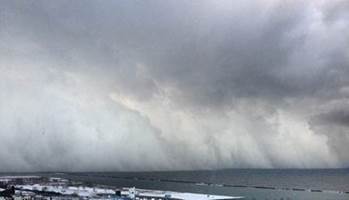
Case 2: Buffalo lake
effect “ Snow Blast”
On November 18, 2014, Buffalo experienced one of the most intense lake effect squalls in history. Images of the wall of snow across Lake Erie are iconic on the Internet:
The radar loop for this case shows a very different reaction than you saw in the Grand Rapids case and the observations show a prolonged period of measureable snowfall.
As
in the first case, you must become familiar with the surface map
for 00Z Nov
18,
surface
map loop,
850 hPa map, 500 hPa vorticity map,
and 250 hPa map.
You also have, as before, the Great
Lakes water
temperatures from Nov 15.
For
this Buffalo case, the resulting lake effect squalls
were very different in terms of intensity as well as structure.
Here are
your questions:
3.
How is the synoptic setup different from the Grand
Rapids case? Wherever possible, be quantitative.
4.
How do these conditions work to create such a
different lake effect event?
5.
Was the forecast guidance (MOS in an Excel
spreadsheet,
and 24
hour
surface prog)
helpful in guiding you
to the correct forecast? Why or why not?
Case 3: Syracuse
2012
In
the Fall of 2012, WxChallenge
chose Syracuse, NY as their northeast
station. Late in the day on Nov 28, radar showed
what
appeared to be a long single lake effect band set up on the south
shore of
Lake Ontario.
Observations
from 12Z Nov 28
to 12Z Nov 29 featured a number of hours with S- but little
accumulation
which may indicate that the long shoreline band was not as strong as it
looked.
You
again have a
surface map loop for the same times as the observations
and, for 00Z Nov 29, the U.S. surface analysis, 850 hPa map, 500 hPa vorticity map,
and 250 hPa map.
The Great
Lakes water
temperatures were from Nov 29. Your MOS digital forecast
was
from the NAM
that
was initialized at 00Z Nov 28, 2012 and the 24 hour
surface prog
was based on the same
00Z initialization.
Please
answer the following:
6. Was this lake effect or not? Justify your answer using the information given.
7. The observations showed 0.00" measurable precipitation. Considering the well-developed long band, how could there be 0 precipitation?
8.
Assess the MOS
guidance for this case, knowing what the observations
were. Would you have made an accurate forecast using this
guidance?
Why or why not?
Send
your text or Word file to
Jerome.Blechman@oneonta.edu by Wednesday,
Nov 8.