Lesson_07.html

Math 277

Elementary Differential Equations

Spring 1999

Dr. Constant J. Goutziers

Department of Mathematical Sciences

goutzicj@oneonta.edu

Lesson 7

Bifurcations

7.1Bifurcations of a one-parameter family of ODE's.

Examples

Example 7.1.1
Sketch a bifurcation diagram for the family . Then find the bifurcation value for this family.

We say that a differential equation that depends on a parameter bifurcates if there is a qualitative change in the behaviour of solutions as the parameter changes. In order to investigate this phenomenon we sketch the equilibrium points of the equation as a function of .

> f:=y->y^2-2*y+mu;

> eq_pnts:=solve(f(y)=0, y);

> plot({eq_pnts}, mu=-3..3, color=red, numpoints=3000);

We see that for there are two equilibrium points, for , there is one equilibrium point and for there are no equilibrium points. We say tha t is a bifurcation value.

In many situations finding y as a function of from the equation f(y) = 0, is a non-trivial proposition. However in most cases the opposite, finding as a function of y proves to be much easier, and the bifurcation diagram can then be generated using a parametric plot. See the following.

> mu_y:=solve(f(y)=0, mu);

> plot([mu_y, y, y=-2..3]);

The exact bifurcation value can be obtained by setting the derivative of mu_y equal to zero.

> mu_bifurcation:=subs(y=solve(diff(mu_y, y)=0, y), mu_y);

>

Example 7.1.2
Consider the modified logistic model with constant harvesting: . The population S and the harvest C are measured in thousands of tons of fish while t is measured in years. Sketch the bifurcation diagram, determine the bifurcation values, and interpret what happens to the solutions as the ha rvest size crosses the positive bifurcation value.

Code the right hand side of the differential equation and use a parametric plot to generate the bifurcation diagram.

> f:=S->3*(1-S/500)*(S/300-1)*S-C;

> equilibrium_equa tion:=f(S)=0;

> hlp:=solve(equilibrium_equation, C);

> plot([hlp, S, S=-100..600], labels=[C, S]);

The bifurcation values are the C-coordinates of the points on this curve with a vertical tangent line. Because the numbers are not "textbook like", we immediately generate decimal approximations.

> S_bif:=fsolve(diff(hlp, S)=0, S);

> bifurcation_values:=[seq(subs(S=S_bif[k], hlp), k=1..2)];

Of course we are interested in the positive bifurcation value. It is here where the system changes from three to one (negative) equilibrium point. This has a fundamental impact on the behaviour of the solutions.

Take for instance a harvesting level of seventy thousand tons per year. This corresponds to a phase line indicated by the blue line in the picture below.

> with(plots):

> p1:=plot([hlp, S, S=-100..600], labels=[C, S]):

> p2:=plot([70, S, S=-100..600], color=blue):

> display([p1, p2]);

Clearly we have two positive equilibrium points, the largest one is a sink and populations close to this sink will stay close to the sink forever. This is easily demonstrated by the following direction field plot.

> deq:=diff(S(t), t)=subs(C=70, f(S(t)));

> with(DEtools):

> DEplot(deq, S(t), t=-10..10, [[S(0)=400]], S=-100..600);

If however, we cross the bifurcation value of an 81.21 thousand t ons per year harvest, then things will go drastically wrong. Suppose for instance we harvest at a rate of ninety thousand tons per year. This corresponds to the magenta phase line in the bifurcation diagram below.

> p3:=plot([90, S, S=-100..600], color=magenta):

> display([p1, p3]);

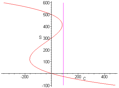
Observe that the positive equilibrium points have disappeared and the population will eventually vanish no matter what its original size. This is nicely demonstrated by the next direction field plot.

> deq:=diff(S(t), t)=subs(C=90, f(S(t)));

> DEplot(deq, S(t), t=-10..10, [[S(0)=400]], S=-100..600, stepsize=0.1, linecolor=gold);

>