Erosion rates in a micro-flume

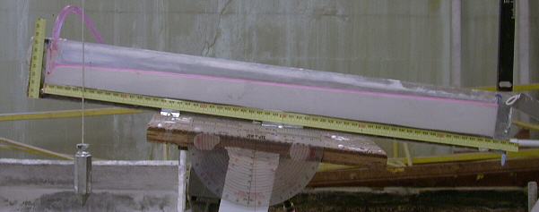
Micro flume, 58.6 cm x 5.6 cm x 0.7 cm (length - height - width), with dye in the flow

Establishing a relationship between flow conditions and erosion rate for my experimental landforms would be very nice to have. It is, however, difficult to obtain quantitative information on flow conditions in the larger basin. I had tried a few dye tracing experiments to get at flow depth, but determining stream width and velocity, or even establishing an overall flow rate at a point on the surface required making a few too many assumptions. I could see that flow depths were very thin, but direct measurement was very nearly impossible. So I resorted to using a very narrow flume, and mimicked the approximate flow conditions in my larger tank.

Ideally, I wanted a relationship between bed shear stress and erosion rate. I started off thinking that I could use a moveable outlet to invigorate erosion in the flume, sprinkle mist over the surface, and measure flow depth, bed surface slope, and integrated flow at the outlet of the flume. During construction, however, I realized I could tilt the flume on a rotating platform and obtain an instantaneous increase in slope over the entire profile. Further, imposing a constant flow rate at the upstream end of the flume simplified the calculation of shear stress. I also wanted a very narrow flume to ensure that the channel width was fixed. More on channel width later...

During initial tests with a small flume, I varied rotation magnitudes at fixed flow rates, and used a substrate of 45 micrometer silica flour (F250 Silcosil). I found, to my delight, that the small size made it very easy to manage. I also discovered that it is very easy to develop knickpoints in the flume by tilting the flume past a critical velocity-depth threshold. In fact, too easy. I wanted to develop a nearly linear bed profile. Knickpoint development and propagation is a very interesting phenomenon to study, but I wanted to get at substrate resistance, without complications surrounding knickpoint dynamics (flow separation, scour, deposition, etc.). For determination of erosion rate as a function of shear stress, I restrained myself to small rotations, and the development of nearly linear profiles.

So, to determine the erosion rate, I took digital photographs from the side of the flume, collected photocoordinates of the bed profile, and converted them to ground coordinates using known ground reference coordinates that appeared in the photo (a simple 2-D conformal transformation). I then numerically integrated the area under the profile over a fixed distance (~90% of the flume length), and divided by the distance to get an average profile height. By differencing sequential average heights, and dividing by separation time, I calculate an erosion rate. I performed this calculation on photographics pairs, one taken immediately after rotation, and another some time later.

To obtain a shear stress requires measurement of bed slope and normal water depth. To get the bed slope, I fit each profile with a linear function to get the profile-averaged slope. I then averaged the slope of the profiles. To obtain the depth, I initially measured the depth of flow with a clear plastic mm scale ruler, guessing to the nearest 0.01 cm. A problem arises here. The water surface develops a meniscus (~0.15 cm) at the wall of the flume. How do I get the depth? I could see from light refraction a bright upper and lower edge to the flow, with a thin clear band of flow between the bright edges. I measured the clear band to the bottom of the lower bright edge. The problem arises for runs conducted at low flow rates, where no clear band appeared on the flume wall. So, I started taking flow depths in the channel center with a point guage--more time consuming but a more precise measurement. These measurements are not normal to the bed--they measure the vertical depth. In order to use depth measurements taken at side of the flume, I measured depth with the point guage and with a ruler on the side of the flume, determined a linear fit between the two methods, and tranformed ruler measurements to point guage measurements. The relation between the two is not very satisfying, and I don't intend to use this method again, but at least it allows me to use measured depths from runs without point guage measurements...I took depth measurements at 10 cm intervals, and averaged the depths.

So, after much averaging, what kind of relation do I get?

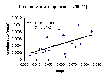
Not a very impressive correlation coefficient. Seems to work for slopes<0.05, but very noisy beyond that.

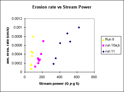
What about stream power? Well, it looks like erosion rates increase with stream power, but again, a rather noisy relation, and with troubling differences in the intercepts and trends between runs (discharge varied between runs: 1.1, 3.5, and 8.4 ml/s for runs 8, 10, and 11 respectively). This is kind of interesting, in that stream power has been proposed as a model for an erosion rate law. Clearly, a different 'law' is required for each discharge. This would seem to limit the applicability of stream power as a universal 'law' for determining erosion rate...

Clearly, slope alone, or slope-discharge product capture some trend, but an additional variable is contoured, if you will, on the stream power diagram. So let's see how bed shear stress for normal flow conditions works...

By golly, Wally, this seems to be the trick! I fit a linear trend to the data points, and out pops the empirical erosion rate law as a function of shear stress...

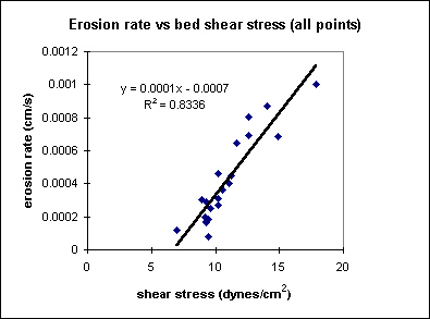
Not by any means a perfect relationship, but not bad considering the measurement errors...The intercept indicates that a critical shear stress is required before erosion begins. Erosion rate appears linear over the range of shear stresses I imposed. The nice alignment indicates that a shear-stress based law for erosion is more universal than stream power.

The flow conditions in the microflume can be characterized by the Froude (velocity/((gravity * depth)^0.5) and Reynolds (velocity * depth / kinematic viscosity) numbers. I report time and space averaged values below for each run above.

Clearly, the flows are laminar, and I definitely pushed run 10 and 11 into a supercritical regime (Fr > 1). Interestingly enough, passing through these different regimes does not appear to affect the erosion rate - shear stress relation. However, like I mentioned above, knickpoints are difficult to keep from spontaneously disrupting the bed profile at supercritical conditions. I still need to determine erosion rates for profiles that developed propagating knickpoints, but that's another project...

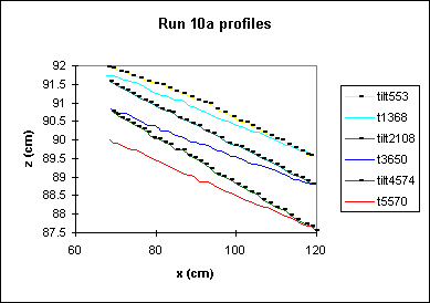
Why all the averaging, you may wonder?! Good question. Conceptually, to get an erosion rate you need to measure a change in elevation at a given point. However, one problem with doing it this way occurred after I opted for rotation as a means of increasing the slope of the bed. I noticed that the bed erodes in a rotational manner, with erosion increasing away from the flume outlet. In this case, erosion rates would increase upstream, even though the slope remained fairly constant along the profile. Hmmmm...So I chose to integrate the profile to get the area under the curve. As soon as you start integrating, you lose local detail, but you do capture ensemble effects. I could, I suppose, devise a flume with a continuously dropping outlet to obtain a uniformly eroding profile. But that seemed to be more effort than I wanted to invest on this problem. It does, however, highlight the difference between forcing a stream with rotation vs base level lowering or block uplift...Below is a figure demonstrating the bed profile response to tilting. The numbers in the legend refer to runtime (in seconds).

Further Work...

Ideally, an erosion law in a flume should be applicable to a erosion in a drainage basin. However, to calculate shear stress in a flow network in a drainage basin requires that some assumptions must be made as to the width of the channel, as well as a relation between depth and slope, or depth and slope-discharge. If a basin is experiencing a constant rainfall-runoff condition, such that flow can be routed and summed through the network, a discharge at a point can be calculated. The local channel slope can also be approximated by the local steepest descent slope. Typically, in numerical models, hydraulic relations between flow depth, width, and velocity to discharge are used to establish the width and depth used in the calculation of shear stress. These relations are based on alluvial rivers, and are fundamentally empirical. Unfortunately, we geomorphologists have still not developed a theory that will yield the width of a channel for various flow and substrate conditions. I would like to incorporate my newly established empirically-derived erosion law in a drainage basin model. Since it is empirical, I may as well proceed with some more empirical relations for depth and flow conditions for the substrate I work with. But those experiments are gonna have to wait...

date constructed: November 30, 2001; last modified: December 5, 2001