Measuring topography is not a trivial problem. Recent technological advances, such as laser altimetry,have made it a tractable problem, but for many scientists with limited resources, it remains a difficult problem. I have tried a few different methods to extract elevation data from my erosion experiments, including a light source/pixel luminance method (failed...), photographs of parallel lines projected on to the ground surface from a slide projector (works, but requires stitching several elevation fields together), and good old fashioned stereophotogrammetry (works, but higher resolution and a metric camera would be nice...). I detail the essential aspects of the photogrammetric method elsewhere. On this page, I detail the processing of the elevation data from xyz points to gridding, and additional processes on the grids...
I start with a set of xyz points that come out of the photogrammetric processing in the ground reference frame of the erosion facility. These points are more or less evenly spaced, because the automated image correlation program steps across a photograph a specified number of pixels. Each correlated point pair, however, is essentially a random pair, because the search algorithm doesn't care about any other correlated points, but just looks +/- a specified search distance along a flight path. The correlations are influenced by the shape of the search box, as well as light variations across the photo that are dependent on that specific photograph alone, such as reflections from water on the surface. While reflections place explicit restraints on the local ground slope, their effect on the correlation process is essentially random, because two photos of the same surface will have differing reflectors, related to the specific geometry of camera, light source, ground location and local ground slope. I have not tried to utilize the geometry of reflections. Instead, I have tried to filter them out.
The basic process from xzy to reported statistics is:
Those of you that have made it this far, and deal with dems, are wondering, "What about the pits?" Ah, the pits. Curse the pits! The processing above takes care of quite a few depressions. The raw grids (7 mm) usually have around 1-3% cells that are depressions. The processing leaves ~0.1 % depressions (~20 depressions in a grid with 12,758 cells). I haven't gone the route of treating the depressions as lakes with a very small slope, and filling them to the lake surface. Any algorithm I could think of did not seem to be controlled or constrained well enough to work in all situations. So up to the present I have largely ignored the pits. I have an algorithm that looks for cells not draining to the depression, and moves flow accumulated in the depression to the lower nearest cell that doesn't drain back to the pit. But I haven't tested it well enough to place much confidence in it.
Why, you may be wondering, get so involved with depressions?! I think there are several reasons for it. One, eroding landscapes have to move material out of the area, and the dominant way this happens is by gravity-driven surface runoff. And unless you're going to argue for reversals in the gravity field with elevation (i.e., water flowing uphill), or dissolution of bedrock causing sinkholes (karst), gravity and surface runoff erosion should never develop a topography with depressions. So it is uncomfortable to my comprehension of erosion that there are depressions in an eroding surface. So there is a physical reason for wanting the perfect downslope convergent flow-path topography to exist-it jives with the concept of runoff based erosion. Tied to this sense of harmony in the landscape is a statistic that is being used extensively these days to calibrate and validate an erosion law based on accumulated flow and local slope. To obtain this statistic, flow must be routed through the landscape. As far as I know, the best and simplest way to do this is to calculate local steepest descent slopes (as a vector), and then travel from every 'cell' on the landscape to the lowest point on the landscape following the local steepest descent. The algorithm I use then, will move so long as the slope is downhill. As soon as it encounters a depression, it stops. It's a simple and robust algorithm, and can find its way through a landscape to the lowest spot so long as there are no depressions. So this is the problem with depressions. And they raise several questions: are they real? are they artifacts from elevation derivation, or the process of gridding xyz data, or from additional processing on the grid? If they're real (and I have been on many a hillslope that has local depressions due to hillslope failure and block rotation, for instance), then well and good, and we shouldn't expect the slope-area statistic to be so perfect. Depressions due to gridding can arise from adjacent cells on ridges separated by a valley that is smaller than the resolution of the grid. Not much we can do here but increase the resolution, but we may find the problem extends down to the smallest scales. We could also move away from evenly spaced gridded data, and develop better vector methods of dealing with topographic data. Evenly spaced gridded data are just so easy to work with, efficient to store and access, and simple to visualize. But maybe there's no other way around the depression problem...
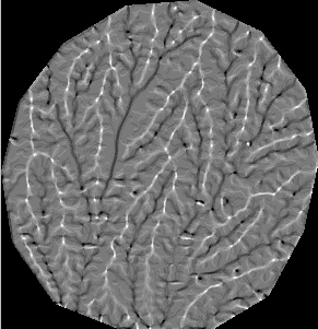
Depressions aside, I have found through working with my own experimental topographic data that processing has a rather significant effect on some geomorphic statistics. I have been trying to compare experimental topography to natural landscape topography (I'll have another page of these comparisons in the future...). So far, the exponent in the slope-upstream area relationship (S = k A^ a) is the biggest difference between natural landscapes and small scale experimental topography. Most reported values of a for natural landscapes are in the range of -0.4 to -0.8. My exponents have all been ~-0.15, though I will show below that the low value may be a processing artifact...I calculated statistics on the same elevation data set that has been processed differently (smoothed vs unsmoothed; gridded at varying spatial resolution, from 3 mm to 15 mm spacing; depression bypassing). The initial xyz data set consists of >100,000 points, and looks like this when read into a screen at roughly 1:1 density (#pts/screen area).
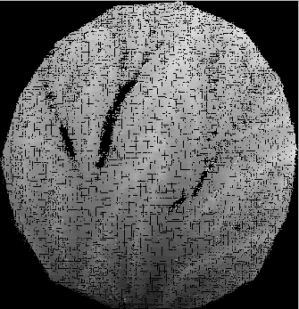
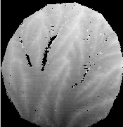
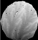
The gray scaled elevation image on the left is 335 x 347 pixels, a spacing of 2.6 mm/pixel. The dark patches are 'no data' cells, and by comparison with the reduced resolution photo on the right, mostly result from reflections.The following images display the changes in appearance with resolution.
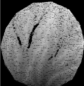
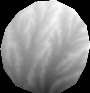
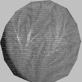
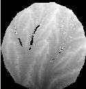
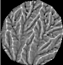
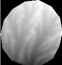
grid without filtering; grid with extreme slopes filtered; grid smoothed once; grid smoothed 3 times
.jpeg)
.jpeg)
.jpeg)
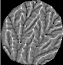
local relative elevation: no filtering 3x3 box; extremes filtered 10x10 box; smoothed 1 time 5x5 box; smoothed 3 times 5x5 box
.jpeg)
.jpeg)
.jpeg)
.jpeg)

.jpeg)
.jpeg)
.jpeg)

.jpeg)

.jpeg)
.jpeg)
.jpeg)

.jpeg)
.jpeg)
.jpeg)
.jpeg)
Well, if you made it this far, Cheers! I'll try to keep this website from narrowing to a single point. Visually, the filtering process has a very pronounced effect on local relative elevation. Filtering the extreme slopes does a pretty good job of getting rid of gross holes or highs. In the absence of smoothing, the structure of the topography only appears in the local relative elevations when the box size increases to a radius of roughly 2.5 cm. 1 pass smoothing really draws out the structure, and 3 passes is visually quite striking, capturing many of the low order valleys.
The raw elevation data set used in the above grid are all derived with a moving cross hair (16 x 16 pixels) correlation, with a search of +/- 6 pixels along the flight line direction after projection. That is, a fixed point in one photo is projected onto the second photo with a 2 dimensional projective transformation. Then the algorithm searches along the flight line for the best correlation. Visually, with some weeding out of extreme slopes, the grids don't look to bad. The advantage of using a cross hair correlation is the large reduction in correlation time. A box can frequently yield slightly better correlations, so if computing time is a not big issue, a moving box might be a preferable means of correlating images. My experience suggests that larger boxes yield smoother initial surfaces. Below is a set of grids from a 20 x 20 pixel moving box, plotted at 7 mm spacing (18,884 initial data points). For comparison, the 7 mm spacing grids from the cross hair correlation are plotted below them. They differences are minor.
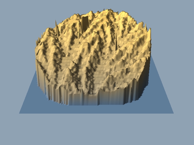
So far, we have been looking at the elevation fields from directly above, which does not afford us a sense of relief. I have been playing with some software that overlays photographs onto elevation grids, and renders them at some angle from vertical as a 3 dimensional object.
Raw 5 mm spacing grid (cross hair correlation)
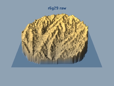
raw 7 mm spacing grid (box correlation)
5 mm spacing with extreme slopes filtered (cross hair correlation)
3d.jpg)
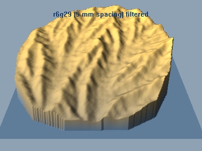
5 mm spacing elevation grid, extremes filtered plus smooth 3x (cross hair correlation)
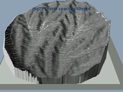
Processed 5 mm spacing with photographic overlay (cross hair correlation)
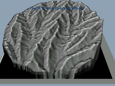
Processed 5 mm spacing with local relative height overlay (cross hair correlation)
From the above visualizations, it is clear that the elevation fields I extract from digital photos at a 1280 x 960 resolution exhibit a lot of roughness prior to processing. The roughness comes from just plain faulty correlations (same patterns but actually different ground locations), from reflections, and 'steppiness' from the relatively low resolution of the digital imagery. Elevation ranges for single pixel shifts during correlation translate into 7-20 mm shifts in elevation, so the derived field is blocky at this scale. Averaging local values yields a more continous appearing surface, but also rounds the ridge crests and any other hard edges in the field. So low resolution limits precise measurement of small scale features such as channel or ridge crest widths, and extracting information about them from the elevation field is a bit sketchy.
I collected elevation, slope, and slope-area distributions from each of the grids at various resolutions, levels of processing, and derived from the correlation methods above, and plotted them together on the same chart to get some sense of the relative importance of these effects have on topographic statistics. Here they are...
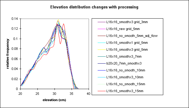
Elevation distributions for various levels of processing and grid spacing
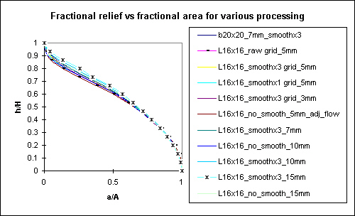
Hypsometric curves (altitude-area) for various levels of processing and grid spacing, asterisk and dash mark the extremes
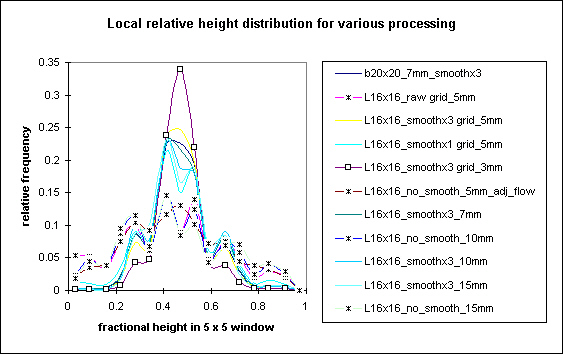
Local relative height distribution for various levels of processing and grid spacing, asterisks denote lack of smoothing
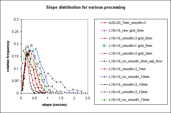
Slope distribution for various levels of processing and grid spacing, asterisks mark non-smoothed data
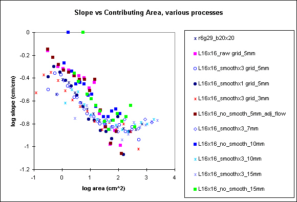
Slope vs Contributing Area for various levels of processing and grid spacing, blocks mark non-smoothed data
Clearly, neither grid spacing nor the level of processing affect the general elevation distributions. The hypsometric curve does not capture much information about the roughness or organized structure of topography. Smoothing the topography, as noted from the imagery plots above, drastically changes the local relative height. The relative height distributions change from very weakly normally distributed plots (the asterisk marks) to very well characterized distributions-the spread of values decrease, the mean approaches a value of 0.5 (i.e., the average grid location has 50% points higher and lower than itself). Interestingly, as this occurs in the frequency distribution, the actual structure of topography also becomes visible in the spatial plot of local relative height. Hmmm...This might be a useful plot. I haven't seen anyone use it in the literature yet, so it may bear further investigation.
Slope distributions are radically affected by the level of processing and by grid spacing. Smoothed topography exhibits a closed form distribution, something like a sin wave with a long tail at large slopes. It's rather difficult to see, but the slope distribution decreases in width for larger grid spacing.
Finally, smoothing has rather non-linear effects on the slope-area relationship. Smoothing decreases slope on the hillslopes and increases slope on downstream sections, generating a relation that looks like a truncated sin wave. Non-smoothed data exhibit a steeper relationship (a ~ -0.3) than smoothed data (a ~ -0.15), that looks somewhat more like a line. I marked the 1 pass smoothing data with a solid dark blue dot. This level of processing maintains a somewhat linear relation (in log-log space, remember), with a ~-0.3.
page last modified June 15, 2001 by Les Hasbargen