Local relative height...What is it?

I'm still sorting out what exactly relative height is telling us. I stumbled across this algorithm when trying to 'visualize' and process gridded data. Essentially, it ranks each point in a grid according to the number of points lower than the point in a moving window (usually 3x3 or 5x5 pixel window). Possible values for relative height are 1 (all nearby points are lower, location is likely to be a peak) to 0 (all nearby points are higher, location is likely to be a depression). The increments of relative height are set by the size of the moving window. For a 3x3 window, the possible values are 0/8, 1/8, 2/8, 3/8 etc., and for a 5x5 window 0/24, 1/24, 2/24 etc. The frequency distribution for local relative height for my miniature landscapes looks like this:

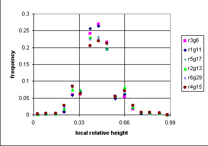
Samples from all runs after complete dissection, 3x3 pixel window (4.41 cm^2 area)in a 7 mm spacing grid, distributions calculated for 8 bins, and

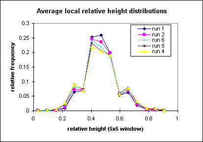
5x5 pixel window in a 7 mm spacing grid (12.25 cm^2 window), distributions calculated for 15 bins

Looks Gaussian to me! Note that the peaks and pits have very small probabilities. The landscape is dominated by points with neighbors that are 50% higher and lower. Expanding the moving window spreads the distribution, and minor peaks show up. I'm not sure if this isn't an artifact of the bin interval (15), or if the secondary peaks are real.

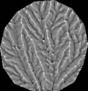
Given that this is just a local ranking algorithm, what good is it, and how useful is it? Like I mentioned above, I have been using it as a visualization tool. When the values of relative height are plotted for elevation grids, visual continuity of spatial features becomes evident. A spatial map of local relative height for run 2 just after complete dissection is shown below in several color levels: gray scale (8 grays, and 255 grays, whites are highs); 8 color scale (red = high, blue = low). Image on left is relative height calculated with a 3x3 pixel moving window (4.4 cm^2 area for 7 mm spacing grid), and the other three are for a 5x5 pixel moving window (6.25 cm^2 area for 5 mm spacing grid).

Obviously, ridges and valleys can be mapped out quite well with this method. What I like about this method is that the fractional area of the basin occupied by ridges and valleys can be easily extracted from the frequency distribution by summing the distribution over the relevant values. Here's the ridge and valley fractional areas for 5 of the runs I have conducted (for run parameter (r/u) values, click here):

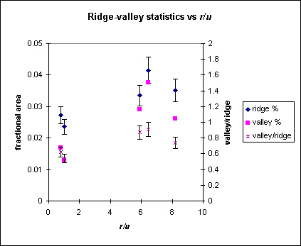
Note that there is a slight asymmetry to the distribution, which is captured by the valley/ridge ratio (right axis). Valley and ridge stats have been extracted from a moving 3x3 pixel window operating on a 7 mm spacing grid. Valleys are sums of the distribution from 0 to 0.33 and ridges summed from 0.66 to 1 (essentially cells with at least 6/8 neighbors higher and 2/8 higher). The measurements indicate that valleys occupy roughly 65-90% of the area that ridges do. Error bars represent the range in measurements for each run (points represent averages). Each grid contained 12,700 points.

And now for some eye-candy. I overlaid relative height onto topography in a land surface visualization program (3DEM)...

Local relative height (255 grays) overlain on the topography (5 mm horizontal spacing)

Local relative height (8 grays) overlain on topography

Local relative height (8 colors, blue-low, red-high)

Observations and Conclusions?