Map of ridge locations (solid black = persistent ridge) through time for an experimental miniature drainage basin forced with constant uplift and rainfall.	Dynamics of Steady-State Drainage Basins: An Experimental Approach	Data in this page is from Les Hasbargen’s PhD thesis (University of Minnesota, 2003).
In recent years geomorphology has experienced a rejuvenation of interest in landscape scale erosion. Landscape evolution modeling has become almost routine, and new models continue to be developed that incorporate greater complexity and feedback between climate, tectonics, and erosion. Our (Les Hasbargen and Chris Paola) approach has been to take a step back, and compare results from the least complicated models with results from a similarly simplified physical experiment. We have built an erosion facility that allows a miniature landscape to erode through several relief distances at constant base level fall and rainfall rates. This kind of experiment permits observation of drainage basin dynamics at steady forcing, offering a view into the internally generated behavior due solely to feedback between stream erosion and transport, and hillslope sediment supply. The landscapes in our basin develop dendritic 3-5 order drainage basins. Dominant erosional processes include stream incision and hillslope failures. We note that knickpoint generation and migration is very common. While it is quite simple to force knickpoint generation with abrupt drops in base level, knickpoints form in our experiments under constant base level fall conditions. The relative activity of erosive processes is sensitive to rainfall and base level fall rates. For instance, rapid uplift (i.e., base level fall) forces larger hillslope failures, and result in larger oscillations in sediment flux leaving the basin. We have conducted 7 runs in the facility thus far. Below you will find a smattering of visual data from the experiments. We collected time lapse video, digital still photographs from stereo locations, and sediment and water flux measurements at the outlet to the basin. All of the runs begin with an initial flat surface with very low surface roughness. The drainage basin forms by headward erosion from the outlet. A rough balance between erosion and uplift (i.e. 'base level fall) is reached shortly after complete dissection of the surface. For runs below, u = uplift rate and r = rainfall rate in mgrams/cm^2/s [L/T]*[M/L^3]; r/u (the water-to-rock ratio) is a dimensionless forcing parameter... A few conclusions from our experimental work... Experimental drainage basins at constant uplift and rainfall rates develop topography adjusted to forcing conditions Mass distribution of topography is sensitive to r/u, with the center of mass moving toward the outlet with increasing r/u Slope (both regional and average steepest descent) decreases with r/u The size of hillslope failures decreases with r/u (no quantitative measurements here yet, but compare run 3 and run 6 time lapse videos...) Knickpoints are common, and give the appearance of upstream propagating waves of erosion Sediment fluxes at steady state erosion vary 10-30% of the long term average Ridges can migrate laterally, extend, shorten, or be annihilated long after a balance between uplift and erosion is achieved Low order (short) ridges are more dynamic than the large ridges, and appear more likely to migrate downstream
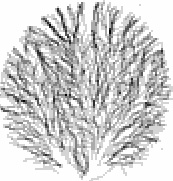
Visual Imagery of Experimental Drainage Basin Evolution Time lapse video of the ground surface, viewed from above the basin (files are cinepak format (*.avi), best viewed with Windows Media Player; VideoLAN, an open source media player, works too: http://www.videolan.org/vlc/index.html) (video info) run 1 ( r/u = 1.0); 20.1 mb (note: surface dryout overnight; shortest eroded distance; best time lapse footage) run 2 ( r/u = 0.8); 21 mb (misty video, but lots of migration) run 3 (r/u = 0.6); 33.9 mb (video ~2/3 of run before camera got wet and fried; large mass movements) run 4 ( r/u = 5); 28.2 mb (run lasted 19 days; highest drainage density of all runs) run 5 ( r/u = 6); entire run, 21 mb; knickpoints late in run, 25.9 mb; (note: major perturbations...) run 6 (r/u = 8); 52.5 mb (most stable forcing of all runs; best documented as well...) run 7 (r/u~2 to 15); 24 mb; spatially variable rainfall, time-varying uplift; yup, sheet flow happens... Still photo sequences (longer duration between images, but higher resolution; *.avi files are rendered better than gif animations, but are bigger files; *.avi best viewed with Windows Media Player) run 1 still photo sequence (617 kb gif)(806 kb, avi) run 2 still photo sequence (350 kb gif )(1.2 mb, avi) run 3 still photo sequence (196 kb gif )(1.94 mb, avi) run 4 still photo sequence (1.1 mb gif)(1.14 mb, avi) run 5 still photo sequence (630 kb gif)(2.45 mb, avi) run 6 still photo sequence (1.6 mb gif)(6.26 mb, avi)
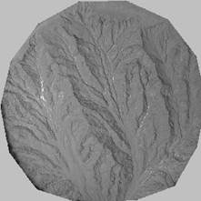
Elevation Time Series, Derived From Stereophotogrammetry Raw elevation animations (gif format) run 1 raw grid 1 fps: 255 grays(73 kb), 8-grays (35 kb); 15 fps: 8-color (35 kb) run 2 raw grid 1 fps 255 grays (129 kb); 1 frame/sec, 8-color (28kb) run 4 raw grid 1 fps (71 kb) run 5 raw grid 2 fps 255 grays (199 kb) run 6 raw grid 1 fps 255 grays (227 kb); 15 fps 255 gray(227 kb); 15 fps 8-color (115 kb) Processed elevation animations (gif format) run 1 elevation 1 fps: 8-color spectra (123 kb) run 2 elevation 1 fps, 8-color (23 kb); 5 frame/sec, 8-color (18 kb) run 4 elevation 2 fps, 8-color (71 kb) run 5 elevation 2 fps 16 grays (41 kb) run 6 elevation 1 fps 16 grays (227 kb); 10 fps 8-color(227 kb) Local relative height animations (gif format) run 1 ridges 1 frame/sec: 255 grays(73 kb), 8-grays (35 kb); 15 frames/sec: 255 gray(73kb); 8-color (35 kb) run 2 ridges 2 frame/sec, 255 grays (71 kb); 2 frame/sec, 8-color (35 kb) run 4 ridges 2 frame/sec, 255 grays (71 kb); 2 frame/sec, 8-color (25 kb) run 5 ridges 2 frame/sec 255 grays (105 kb); 1 frame/sec 8-color (53 kb) run 6 ridges 3 fps 255 grays (227 kb); 3 fps 8-color(227 kb) Spatial erosion rates, derived from differencing gridded elevations (gif format) run 1 8 grays(110 kb);8-color(75 kb) run 2 255 grays (111 kb); 8-color(76 kb) run 4 8-gray(94 kb); 8-color (64 kb) run 5 1 fps 255 grays (68 kb); 1 fps 8-color (47 kb) run 6 1fps 255 grays (666 kb); 1 fps 8-color(267 kb) Elevation Data as simple text files, as gridded or vector (x,y,z) data; note the letter ‘g’ in the file name indicates a group of photos taken during the run used to generate the elevation data. The links will take you away from the SUNY Oneonta server to Google Drive. Includes sediment flux, run conditions, ground control for photos, substrate mix, etc for each run. run 1 run 2 run 3 run 4 run 5 run 6
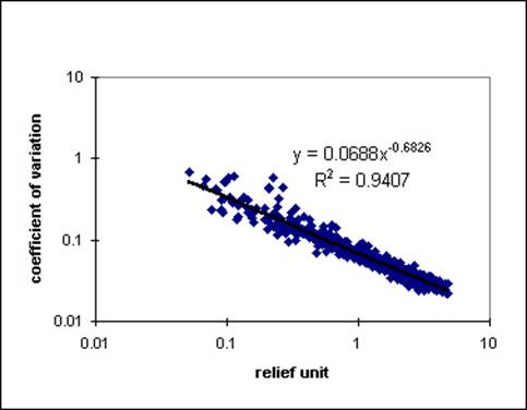
Spatial and temporal statistics of experimental landscapes Erosional variance (standard deviation of erosion rate / average erosion rate) vs eroded distance (relief unit is maximum relief at steady forcing). Clearly, erosion rate variability is quite large at short observation time scales.
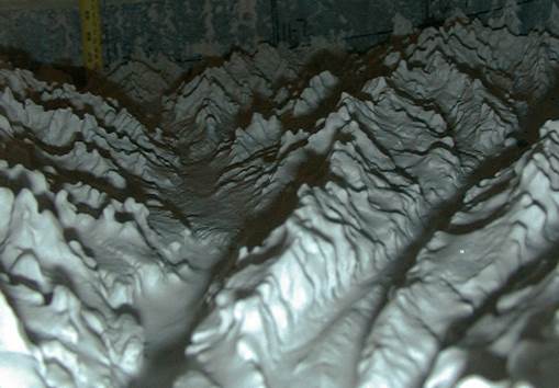
Pretty pictures of the basin from a lower angle...
Numerical models of Eroding Landscapes I have written into code a couple of the published landscape evolution models out there (Howard, 1994; Chase, 1991), to get some sense of the kind of erosional behavior one might expect from them. See Alan Howard’s excellent page in landscape erosion modeling. I modified Howard's model to my own ends...Some of the changes are to the numerical lattice boundaries. I set a single outlet for eroded material to exit the lattice, and enforced a planform boundary to the lattice similar to my physical sandbox experiment. I also modified processes operating on the numerical lattice, such as erosion based on stream curvature, hillslope failure, and directional diffusion. For more details on erosional processes, see information on the model used to make these animations. Model animations (time series of gray scale elevation fields) R2 upstream area + diffusion + periodic uplift (gif animation 414 kb)(input parameters) R9 upstream area +diffusion (gif animation 475 kb)(input parameters) R12 upstream area +diffusion (gif animation 664 kb)(input parameters) R13 upstream area +slope failure (gif animation 682 kb)(input parameters) R 18 upstream area + stream curvature (gif animation 681 kb)(input parameters) R22 slope failure only (gif animation 376 kb)(input parameters) R27 upstream area + stream curvature (gif animation 670 kb)(input parameters) R29 upstream area + asymmetric diffusion (gif animation 662 kb)(input parameters) R30 upstream area + asymmetric diffusion (gif animation 645 kb and 304 kb-4_color)(input parameters) A few conclusions... · While the numerical simulations exhibit lateral migration of ridges/streams, this behavior dies out as some (for lack of a better term) optimal network is achieved. All of the simulations I have run are driven to this stable form (though some of the simulations clearly were not run long enough...). Stability is achieved shortly after a balance between erosion and uplift has been established, and usually not more than a relief's worth of erosion beyond complete dissection of the initial surface (Howard notes a limit of 3 reliefs to achieve stability). · When ridges do migrate, they appear to 'close' from the upstream to the downstream end. · Adding additional terms to the erosion law, such as for stream curvature, for threshold slope driven slope failures, or general diffusion, does not lead to self-sustaining migration. Numerical Model runs last updated June 11, 2001 by Les Hasbargen
page last modified October 11, 2013 by Les Hasbargen Email: Leslie.Hasbargen@oneonta.edu Dept. of Earth & Atmospheric Sciences State University of New York, College at Oneonta Les’ web site: http://employees.oneonta.edu/hasbarle/ Les is solely responsible for the content in this web site.