Space-Time Measures of Erosion Dynamics
I have spent a fair amount of time looking at the time-lapse videos of the experimental landforms. I am always struck both by the sense of similarity during the course of each run, and upon closer inspection, the vigor of migration at small and intermediate scales in the basin. Responses I have gotten from various people who have looked at the videos range from 'Hmm...Looks stable to me.' to 'Wow, The landscape is alive!' and 'It looks like it [the landscape] is breathing!'. How does one characterize such a system?
I am still learning different ways (mathematical, mostly) that others have used to describe system behavior, as well as trying to imagine ways that I find simple (I'm not a sophisticated boy...) and useful. When dealing with a system, it's helpful to start with constant forcing at the boundaries, such as heating a pot of water uniformly at the base, and cooling it uniformly at the surface, or doing a similar experiment with a solid chunk of copper, or even growing a plant with uniformly supplied nutrients and light. Obviously, the material being forced plays a big role in how the heat (or energy) arrives at the far boundary. A pot of water boils, advecting heat and developing a full blown circulation, whereas a copper solid diffuses heat in a more uniform fashion. I suspect that my eroding sandbox is somewhere between the two...
So far, I have thought about my erosion experiments in terms of stability. Do the planform features (ridges and valleys) vary over the course of a run, especially after a regional slope has developed, and flow paths are well-defined? If so, are the features statistically stable, i.e., do ridges occupy a constant area within the basin? If there is movement of features, is it random and localized, or is movement propagating through the network? Do perturbations propagate through the basin? If so, are they dampened or amplified as they move through the basin? Does the system develop stabilizing feedback? I imagine the worst case scenario for describing a system is that the answer to all of the above questions is 'yes'.
It is clear to me that we are dealing with a self-organizing system. I do not impose the location of ridges and valleys, nor do I prescribe when and where a hillslope will fail and slump into a stream. I only feed it rain and lower its base level, and it takes over from there. It is also clear that there is migration of ridges and valleys, but within a statistically stable (i.e., a well-defined average) framework of regional and local slope.
As initial measures on the time-space varying nature of experimental landforms, we calculated a few statistics based on a time series of gridded elevation data: variance of erosion rate vs time, variance of erosion rate vs space, average flow direction change vs time, and number of cells with flow direction changes vs time.
Erosion rate variability and observation time scale...
Erosion rate animations exhibit rather hard to decipher, or at least, hard to characterize, spatio-temporal patterns (back to erosion rate videos). Erosion appears to be rather local, with smaller subregions experiencing increased erosion at any one time. So, when dealing with complexity, average, average, average...Which in this case, means that we calculated the average and standard deviation of erosion rate for all possible time lags between gridded data sets, and plotted the standard deviation divided by the mean erosion rate (coefficient of variation) against the lag spacing (i.e., time) between sets. Intuitively, for very large vertical distances between data sets, where the average distance is much greater than the local variance of elevation, this ratio must approach zero. Fortunately, intuition holds this time. We also hoped to get a characteristic time scale for each time series. However, it appears that the relationship between the coefficient of variation and lag spacing is a power law.
Charts 1 and 2 Erosion rate variance plotted against observation time for Run 2
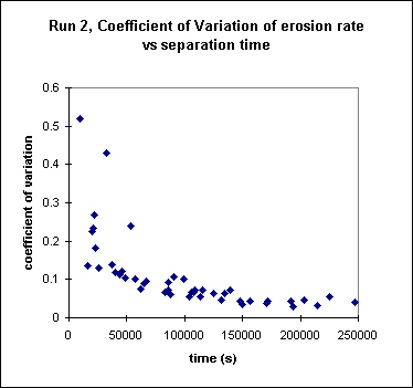
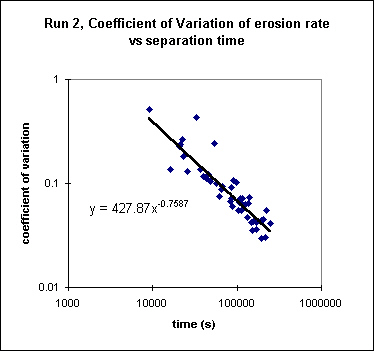
The first image is a plot of the coefficient of variation vs lag spacing, and the second is plotted in log-log space, which straightens the first plot quite nicely.
However, plotting a dimensionless variable against a dimensional one is not all that useful for generalizing results (Who measures erosion rates in seconds? Aside from me...). We can replace time with distance in this case, and scale that length to the relief of the system. So, we transform time separation between grids into a dimensionless fraction of eroded relief by multiplying the time separation by uplift rate, and dividing by the average maximum relief. Uplift rate * time works in this case, because uplift rate is constant. One could also take the difference between the minimum elevation at two times, and divide this length by the maximum relief to get the same answer.
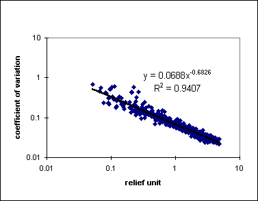
The plot below shows that erosion rate variance increases at smaller separation times, or equivalently, eroded relief. This plot is significant because the data are taken from 5 experimental landforms that are balancing uplift with erosion (dynamic equilibrium), all with different uplift and rainfall rates. One might think (in fact, many geomorphologists have assumed) that at dynamic equilibrium, streams and hillslopes are delicately adjusted to each other, and the landform erodes everywhere at the same rate. Numerical simulations of landscape evolution have supported that idea (see numerical animations). Our physical experiments suggest that only over very long times (after eroding through the relief of the landscape) will the spatial variance of erosion approximate the long term average. There is a lot of local variance in erosion rates when viewed at shorter time scales...
.jpeg)
We fit power law equations to the above data sets, and find that exponents for all data sets range from -0.68 to -0.76, a rather narrow range. This suggests that the spatial variance of erosion rate is not directly linked to forcing conditions (and hence, erosional processes), but may actually be the signature of the erosional style for dendritic landscapes in general. Below is a plot of data from 5 runs, with the average power law exponent (~-2/3).
Erosion rate variability and observation spatial scale...
The plot above demonstrates how erosion rate variability changes through time. What about variability across space? That is, if we look at variability over larger areas, is the variability the same regardless of the size of the area? Is our scale of observation giving us a biased view of variability? For the variability (the coefficient of variation, standard deviation divided by average) to be the same at any observation scale, the average must be well-defined at all scales. From a statistical point of view, this becomes less likely at smaller areas, as the number of data points decreases for smaller areas. This certainly holds for gridded data sets. (Wouldn't it be nice to have densely packed data at all scales?! Too expensive for most budgets...especially mine.) Anyway, it makes sense that the average may not be well-characterized at small scales, and as you incorporate more data, the average becomes more stable. Now, if the variability is the same at all scales, we have a fractal. A plot of variability against the scale of observation (area, in our case) would be a flat line. In this case, the measure of fractality tells us that the object we are plotting fills space. What if the line is not flat, but sloping? Our variability is changing with observation scale, and the object is still fractal, but less so. If we plot our data in log-log space, and the data fall on a straight line, we have a power law (y = a * x^b), where 'b' (the exponent) is the slope of the line. Mark and Aronson (1984) have shown that the degree of fractality (the fractal exponent) is related to the exponent b in a power law relation as D = 3-2*b, where D is the fractal exponent.
So, I would like to know, is a sandbox drainage basin fractal? To answer this question, I used two different methods that quantify variability--the semi-variogram, which plots the squared difference of a value against the distance between values; and lacunarity, which calculates the coefficient of variation (standard deviation/mean) against the area over which the mean and standard deviation have been calculated. The semi-variogram (plotted as an omnidirectional variogram) for an elevation data set (~40,000 x,y,z data points) for run 2 looks like this:
.jpeg)
If the line is straight, I would have a simple fractal. In this case, there is a pronounced curvature to the relation. At short length scales, the very low slope to the relation suggests that the elevation field is highly fractal (D ~2.7), and at long length scales, the fractality decreases. I have a multifractal. Arghh! It's not a term I am very happy with. The break in the two main trends is somewhere around 10 cm, which is about the hillslope length of the main ridges for run 2. The roughness of the surface (or the noise in the data) is reflected by the intercept at a distance = 1 cm, with a variance ~3-4 cm^2, or a standard deviation ~1.5-2 cm. This is on the order of the errors in deriving elevation using low resolution digital imagery (1280 x 960 pixels).
For lacunarity analysis, I followed Plotnick et al. (1996), only I modified the sliding box algorithm to a Monte Carlo subsampling of points on a grid of elevation. I did this because using a sliding window greatly increases computation time as the box size increases. Plots of sliding box vs subsampling were very similar, so I used the subsampling method, with 200 random locations in the grid selected for the calculation of the mean and standard deviation at each window size, which I varied from 9 pixels to 1600 pixels. Here's what the relation between the coefficient of variation and box area looks like:
.jpeg)
I performed the calculation on two test grids, just to get some idea of what this algorithm captures. The 'funnel slope (rnd)' plot is for a grid of elevations that increase linearly from a point, with minor noise added to the data. A visualization of this grid would look like a rough funnel. 'Random field' is exactly that, an evenly distributed set of random elevations in a grid. Again, straight line plots are signs of a single fractal exponent. The random field plots as a fractal (D = 2). So do 'ridges' and, to a lesser degree, 'slope' data sets. Slope is the slope magnitude in the steepest descent direction, and 'ridges' is the local relative height. Elevation fields ('raw grid' and 'filtered grid'), 'streams', 'erosion rate' and 'funnel slope' exhibit breaks in the relation, somewhere around 50-100 cm^2. 'Streams' is the upstream area draining through a point on the grid, and 'erosion rate' is the local erosion rate derived by difference sequential elevation grids, and dividing by the separation time. 'Streams' and 'erosion rate' plot quite closely to each other, which is rather curious. I'm not quite sure what to make of this yet, though it would suggest that upstream area (i.e., stream locations) may be responsible for variability in erosion rate.
One last plot. I calculated lacunarity for several possible time lags of erosion rate for run 2. I was hoping they would all fall on top of each other, or at least, show systematic shifts related to the time lag. They do fall within a rough region, but they don't show a trend with time lag...Note that I again rescale time separation into the fraction of maximum relief.
.jpeg)
The plots all show a break in the trend ~30-50 cm^2. If I ignore that break for now, and fit a power law to the trend, the exponent is ~-1/3. Hmmm...I now have power law exponents for erosional variability in space and time. Since area = distance^2, I can plug distance (L) into the relation: variability ~ A^-1/3 ~ (L^2)^-1/3 ~ L^-2/3, and find that time variability scales directly with space (rather, distance) variability. Very curious. If this is right, than I have experimental evidence supporting the idea that we can substitute space for time in eroding drainage basins, the classical ergodic reasoning approach when time series are not available, but we suspect nonetheless that a landform may exhibit a characteristic form at different times in its evolution. Very curious....
Flow direction changes at dynamic equilibrium
Another measure of spatio-temporal erosion dynamics is the constancy of flow paths. I did some numerical erosion simulations some years ago, where I was trying to figure out what controls re-excavation of buried valleys. Will streams always reoccupy an old valley? Sounds esoteric and unusual, but here in Minnesota we have fairly large areas with completely buried ridge-and-valley networks. Anyway, I wanted to compare the evolving surface topography to one that I had buried. I realized that two surfaces must be identical if flow directions and slope magnitudes were the same on a point-by-point basis. Chris Paola pointed out that the dot product is a convenient tool for measuring angles between vectors. So then, flow direction change is calculated by taking the dot product of steepest slope direction unit vectors on a cell by cell basis between two data sets, summing the dot products, and dividing by the number of cells. Values of 1 imply exactly similar flow fields; -1 indicates complete flow reversal (topographic inversion). We ignored slope magnitude in the calculation, except to use the steepest descent to find the flow direction. The plot below shows that indeed, flow directions are changing in our experiments. At short separation times, grids exhibit a high degree of similarity. At longer times, changes in flow direction accumulate, and grids become less recognizable. For run 6, the flow field has rotated on average cos(a) = 0.3, or 72 degrees, at large lag times. Quite remarkable, considering that a mean flow direction is imposed by having a single outlet to the erosion facility.
.jpeg)
Curiously, transforming time separation into eroded relief does not bring the different data sets into exact coincidence, such as occurred for the spatial erosion rate variance plot. Run 2 appears to reach a limit to flow direction changes that is different from run 4, which in turn is different from run 6. Plotting these data in log-log space seems a bit sketchy, given that flow change, an angular measure, can only vary between -1 and 1, leaving little room for decades in log space. But here's the plot...
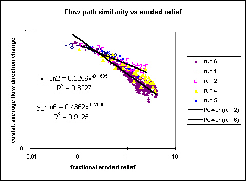
The power law exponent varies quite a bit between the two data sets (runs 2 and 6), suggesting that flow change is sensitive to forcing conditions and hence, erosion processes. Run 6, which does not have obvious hillslope failures (back to time-lapse videos), is accumulating changes in average flow direction faster than run 2 (which had a lot of slope failures).
One last chart to chew on...I counted the number of cells in the grid with flow direction changes greater than some angular threshold, and normalized this number to the total number of cells in the grid, and plotted this fraction against eroded relief. I did this for a couple of threshold angles (44 and 89 degrees). 45 degrees is the smallest nonzero directional change I can compute in a cell that looks to its eight adjacent neighbors. Here's what that plot looks like...
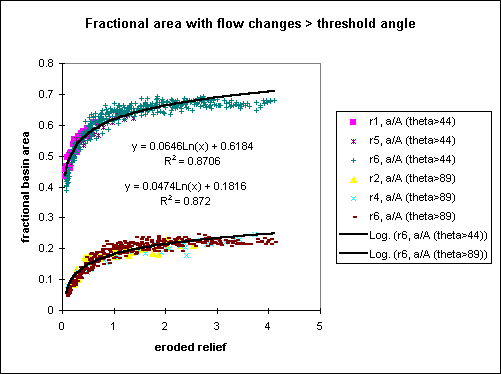
The dependence on run conditions disappears for this measure (runs plot on top of each other). For either threshold, the number of cells increases with time separation up to a well-defined limit. For flow direction change >44 degrees, this limit is about 2/3 of the total basin area. For a threshold of 89 degrees, this limit is ~1/5 of the basin area. For both thresholds, the limit is reached (approximately) at 1 unit of eroded relief.
page first developed October 13, 2001; last modified January 23, 2002 by Les Hasbargen